向量檢索是整個RAG管道的一個重要的步驟，傳統的暴力最近鄰搜索因為計算成本太高，擴展性差等無法應對大規模的搜索。

HNSW（Hierarchical Navigable Small World，分層可導航小世界圖）提供了一種對數時間複雜度的近似搜索方案。查詢時間卻縮短到原來的1/10，我們今天就來介紹HNSW算法。

傳統搜索方法在高緯度下會崩潰，並且最近鄰搜索（NNS）的線性時間複雜度讓成本變得不可控。HNSW圖的出現改變了搜索的方式。它能在數十億向量上實現對數複雜度的實時檢索。但大多數工程師只是把它當黑盒用，調調

efSearch

和

M

參數，並不真正理解為什麼它這麼快，也不知道如何針對具體場景做優化。

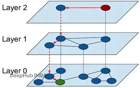
HNSW為什麼這麼塊

HNSW的效率來自概率連接和受控探索。兩個超參數決定了性能權衡：

M（連接度）：決定每個節點的鏈接數量。M越大準確率越高，但內存佔用和索引時間也會上升。

efSearch（動態搜索廣度）：控制查詢時探索的候選數量。更高的efSearch帶來更好的召回率，但是會有更大的延遲。

低延遲實時系統（聊天機器人檢索、推薦引擎推理）適合用小M（8-12）配合小efSearch（32-64）。批量分析或高召回率RAG管道可以用大M（32+）和大efSearch（200-400），在可控成本下得到接近精確的結果。

調優得當的HNSW索引，在中等規模數據（1000萬到1億向量）上能超過FAISS IVF-PQ，維護成本還更低。

掌握HNSW不僅要知道默認配置，而且還要理解它的動態特性。

可視化各層結構。用平均節點度、層佔用率這些指標識別不平衡。

測量召回率-延遲曲線。在不同efSearch值上跑基準測試，找到你的工作負載的帕累託前沿。

優化內存佔用。索引大小按O(M × N)增長，精度允許的話用float16嵌入。

結合量化壓縮。超大規模系統可以把HNSW和乘積量化（PQ）混用，壓縮內存的同時保持召回率。

代碼實現詳解

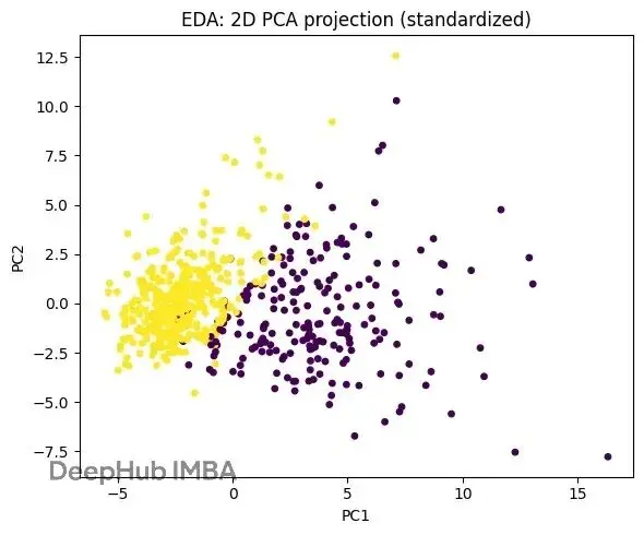
這個腳本演示瞭如何用HNSW替代UCI乳腺癌數據集上的暴力k-NN。完整流程包括：加載數據，用2D PCA做快速EDA揭示聚類結構，標準化特徵，可選地應用PCA生成緊湊嵌入（基於距離的方法對尺度很敏感）。

自定義的

HNSWClassifier

封裝了hnswlib庫。fit階段構建分層小世界索引（由M和ef_construction調優），預測時用可控廣度ef_search檢索k個近似鄰居，投票決定分類標籤。代碼對(M, ef_search, k)做交叉驗證找高F1低延遲的操作點，然後在訓練集上訓練，在測試集上評估。還使用了對照組跑暴力k-NN基線來量化速度和質量。最後通過掃描ef_search可視化帕累託曲線（展示延遲如何上升而準確率趨於平穩），畫混淆矩陣。所有邏輯都包在

run_hnsw_benchmark()

函數裏，一次調用就能跑完整個流程。

 """  
HNSW in Practice — End-to-end example on a real UCI dataset (Breast Cancer Wisconsin)  
---------------------------------------------------------------------  

這個單文件腳本演示瞭如何使用HNSW（通過`hnswlib`）作為一個快速、高召回率  
的近似最近鄰（ANN）引擎來*替換暴力k-NN*在分類工作流程中。它連接了  
從文章核心思想——"非結構化空間中的結構化搜索"——到具體、可重現的  
在廣泛可用的基準數據集上的步驟。  

我們註釋每個階段並解釋不僅*做什麼*，而且*為什麼*對從業者重要。  

依賴：  
    pip install hnswlib scikit-learn matplotlib numpy scipy  

運行：  
    python hnsw_hands_on.py  
"""  

# ======================  
# PHASE 0 — Imports  
# ======================  
# Why: We gather the scientific Python stack, sklearn utilities, and hnswlib for HNSW ANN search.  
import time  
import math  
import warnings  
from dataclasses import dataclass  
from typing import Dict, Any, Tuple, List  

import numpy as np  
import matplotlib.pyplot as plt  

from sklearn.datasets import load_breast_cancer  
from sklearn.preprocessing import StandardScaler  
from sklearn.decomposition import PCA  
from sklearn.model_selection import StratifiedKFold, train_test_split  
from sklearn.metrics import (  
    accuracy_score,  
    f1_score,  
    classification_report,  
    confusion_matrix,  
)  
from sklearn.neighbors import KNeighborsClassifier  

try:  
    import hnswlib  # Fast C++ ANN library with HNSW  
except ImportError as e:  
    raise SystemExit(  
        "此示例需要hnswlib。\n使用以下命令安裝：pip install hnswlib"  
    ) from e  

# ======================  
# Utility Data Structures  
# ======================  
@dataclass  
class CVResult:  
    params: Dict[str, Any]  
    mean_f1: float  
    mean_acc: float  

# ======================  
# PHASE 1 — Data Loading  
# ======================  
# Why: We use a *real* benchmark (UCI Breast Cancer Wisconsin), bundled in scikit-learn.  
# It's binary, tabular, and has enough dimensionality to show ANN benefits without GPU.  
def load_data() -> Tuple[np.ndarray, np.ndarray, List[str]]:  
    data = load_breast_cancer()  
    X = data["data"]  # shape (n_samples, n_features)  
    y = data["target"]  # 二元標籤：0 = 惡性，1 = 良性  
    feature_names = list(data["feature_names"])  
    return X, y, feature_names  

# ======================  
# PHASE 2 — EDA (Quick)  
# ======================  
# Why: In an ANN pipeline, we care about scale/distribution because distance metrics are  
# sensitive to feature magnitudes. Quick EDA guides our choice to standardize and optionally reduce dim.  
def quick_eda(X: np.ndarray, y: np.ndarray, feature_names: List[str]) -> None:  
    print("\n=== EDA: 基本信息 ===")  
    print(f"樣本數：{X.shape[0]}，特徵數：{X.shape[1]}")  
    unique, counts = np.unique(y, return_counts=True)  
    class_dist = dict(zip(unique, counts))  
    print(f"類別分佈（0=惡性，1=良性）：{class_dist}")  

    # Visualize first two principal components to *reason about* structure.  
    # Why: Low-dimensional projection lets us see clusters and overlap, which affect k-NN behavior.  
    with warnings.catch_warnings():  
        warnings.simplefilter("ignore", category=RuntimeWarning)  
        pca_2d = PCA(n_components=2, random_state=42).fit_transform(StandardScaler().fit_transform(X))  

    plt.figure(figsize=(6, 5))  
    plt.title("EDA: 2D PCA投影（標準化）")  
    plt.scatter(pca_2d[:, 0], pca_2d[:, 1], c=y, s=15)  
    plt.xlabel("PC1")  
    plt.ylabel("PC2")  
    plt.tight_layout()  
    plt.show()  

# ======================  
# PHASE 3 — Feature Engineering  
# ======================  
# Why:  
#  - Standardization: Euclidean distances underpin HNSW's "l2" metric. Scaling avoids dominance by high-variance features.  
#  - Optional PCA: Reduces noise and may improve neighborhood quality and latency. It's a trade-off:  
#    too aggressive PCA can hide discriminative detail; modest reduction can help ANN structure.  
def make_embeddings(  
    X_train: np.ndarray, X_test: np.ndarray, n_pca: int = None  
) -> Tuple[np.ndarray, np.ndarray, StandardScaler, PCA]:  
    scaler = StandardScaler()  
    X_train_scaled = scaler.fit_transform(X_train)  
    X_test_scaled = scaler.transform(X_test)  

    pca_model = None  
    if n_pca is not None:  
        pca_model = PCA(n_components=n_pca, random_state=42)  
        X_train_emb = pca_model.fit_transform(X_train_scaled)  
        X_test_emb = pca_model.transform(X_test_scaled)  
    else:  
        X_train_emb = X_train_scaled  
        X_test_emb = X_test_scaled  

    print(  
        f"嵌入維度：{X_train_emb.shape[1]} "  
        f"（PCA={'開啓' if n_pca else '關閉'}）"  
    )  
    return X_train_emb, X_test_emb, scaler, pca_model  

# ======================  
# PHASE 4 — Model Selection: HNSW k-NN Classifier  
# ======================  
# Why: HNSW provides a *hierarchical small-world graph* over points. Search descends coarse-to-fine  
# layers, approximating nearest neighbors with logarithmic scaling—key to fast retrieval at scale.  
#  
# We'll implement a lightweight k-NN classifier on top of HNSW by majority vote over neighbors.  
class HNSWClassifier:  
    def __init__(  
        self,  
        space: str = "l2",  
        M: int = 16,  
        ef_construction: int = 200,  
        ef_search: int = 64,  
        k: int = 5,  
        random_state: int = 42,  
    ):  
        self.space = space  
        self.M = M  
        self.ef_construction = ef_construction  
        self.ef_search = ef_search  
        self.k = k  
        self.random_state = random_state  

        self.index = None  
        self.labels = None  
        self.dim = None  

    def fit(self, X: np.ndarray, y: np.ndarray):  
        n, d = X.shape  
        self.dim = d  
        self.labels = y.astype(np.int32)  

        # Build HNSW index  
        self.index = hnswlib.Index(space=self.space, dim=self.dim)  
        # 'init_index' builds the topological skeleton. ef_construction controls graph quality/speed.  
        self.index.init_index(max_elements=n, M=self.M, ef_construction=self.ef_construction, random_seed=self.random_state)  
        self.index.add_items(X, np.arange(n))  
        self.index.set_ef(self.ef_search)  # ef_search controls query-time breadth (recall vs latency)  

    def predict(self, Xq: np.ndarray) -> np.ndarray:  
        # Query k approximate neighbors for each vector; majority vote on labels.  
        # NOTE: For binary, we could also weight votes by inverse distance.  
        labels_idx, distances = self.index.knn_query(Xq, k=self.k)  
        # labels_idx: (n_queries, k) -> indices into self.labels  
        yhat = []  
        for neigh in labels_idx:  
            votes = np.bincount(self.labels[neigh], minlength=np.max(self.labels) + 1)  
            yhat.append(np.argmax(votes))  
        return np.array(yhat)  

    def predict_proba(self, Xq: np.ndarray) -> np.ndarray:  
        # Simple probability from neighbor class frequency (can be replaced by distance weighting).  
        labels_idx, distances = self.index.knn_query(Xq, k=self.k)  
        n_classes = np.max(self.labels) + 1  
        probas = np.zeros((Xq.shape[0], n_classes), dtype=float)  
        for i, neigh in enumerate(labels_idx):  
            votes = np.bincount(self.labels[neigh], minlength=n_classes).astype(float)  
            probas[i] = votes / (votes.sum() + 1e-12)  
        return probas  

# ======================  
# PHASE 5 — Hyperparameter Tuning with Cross-Validation  
# ======================  
# Why: HNSW has two critical controls:  
#  - M: graph connectivity degree (memory & index-time vs accuracy)  
#  - ef_search: query breadth (latency vs recall/accuracy)  
# We tune them (and k) using Stratified K-Fold to locate a Pareto-efficient setting.  
def hnsw_cv_tuning(  
    X: np.ndarray,  
    y: np.ndarray,  
    param_grid: Dict[str, List[Any]],  
    n_splits: int = 5,  
    n_pca: int = None,  
    random_state: int = 42,  
) -> CVResult:  
    skf = StratifiedKFold(n_splits=n_splits, shuffle=True, random_state=random_state)  
    results: List[CVResult] = []  

    # Small, principled grid: balances realism (we'd try more) and time.  
    grid_list = []  
    for M in param_grid.get("M", [16]):  
        for efc in param_grid.get("ef_construction", [200]):  
            for efs in param_grid.get("ef_search", [32, 64, 128]):  
                for k in param_grid.get("k", [5]):  
                    grid_list.append(dict(M=M, ef_construction=efc, ef_search=efs, k=k))  

    print(f"\n=== HNSW CV調優：{len(grid_list)}個配置，{n_splits}折 ===")  
    for cfg in grid_list:  
        fold_f1, fold_acc = [], []  
        for train_idx, val_idx in skf.split(X, y):  
            X_tr, X_val = X[train_idx], X[val_idx]  
            y_tr, y_val = y[train_idx], y[val_idx]  

            # Feature pipeline per fold to avoid leakage  
            X_tr_emb, X_val_emb, _, _ = make_embeddings(X_tr, X_val, n_pca=n_pca)  

            clf = HNSWClassifier(  
                space="l2",  
                M=cfg["M"],  
                ef_construction=cfg["ef_construction"],  
                ef_search=cfg["ef_search"],  
                k=cfg["k"],  
                random_state=random_state,  
            )  
            clf.fit(X_tr_emb, y_tr)  
            y_pred = clf.predict(X_val_emb)  

            fold_f1.append(f1_score(y_val, y_pred))  
            fold_acc.append(accuracy_score(y_val, y_pred))  

        res = CVResult(params=cfg, mean_f1=float(np.mean(fold_f1)), mean_acc=float(np.mean(fold_acc)))  
        results.append(res)  
        print(f"配置 {cfg} -> F1: {res.mean_f1:.4f} | Acc: {res.mean_acc:.4f}")  

    # Select best by F1 (can also break ties by accuracy or latency measurements)  
    best = max(results, key=lambda r: (r.mean_f1, r.mean_acc))  
    print(f"\n最佳HNSW CV參數：{best.params}（F1={best.mean_f1:.4f}，Acc={best.mean_acc:.4f}）")  
    return best  

# ======================  
# PHASE 6 — Baseline (Brute Force k-NN) for Comparison  
# ======================  
# Why: As practitioners, we need to *quantify* what HNSW buys us. k-NN (brute) is the canonical baseline.  
def brute_knn_baseline(  
    X_train_emb: np.ndarray,  
    y_train: np.ndarray,  
    X_test_emb: np.ndarray,  
    y_test: np.ndarray,  
    k: int = 5,  
) -> Dict[str, Any]:  
    t0 = time.perf_counter()  
    knn = KNeighborsClassifier(n_neighbors=k, algorithm="brute", metric="euclidean")  
    knn.fit(X_train_emb, y_train)  
    train_time = time.perf_counter() - t0  

    t1 = time.perf_counter()  
    y_pred = knn.predict(X_test_emb)  
    query_time = time.perf_counter() - t1  

    acc = accuracy_score(y_test, y_pred)  
    f1 = f1_score(y_test, y_pred)  

    return {  
        "model": knn,  
        "acc": acc,  
        "f1": f1,  
        "train_time_s": train_time,  
        "query_time_s": query_time,  
        "k": k,  
    }  

# ======================  
# PHASE 7 — Train Final HNSW, Evaluate, and Visualize Trade-offs  
# ======================  
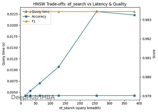
# Why: After selecting params, we fit on train and test on hold-out. We also *sweep ef_search*  
# to visualize the core speed-recall dial that defines HNSW's value proposition.  
def fit_eval_hnsw_and_visualize(  
    X_train: np.ndarray,  
    y_train: np.ndarray,  
    X_test: np.ndarray,  
    y_test: np.ndarray,  
    best_cfg: Dict[str, Any],  
    sweep_ef_search: List[int],  
) -> Dict[str, Any]:  
    M = best_cfg["M"]  
    efc = best_cfg["ef_construction"]  
    k = best_cfg["k"]  

    # Train with best ef_search for final scoring  
    efs_final = best_cfg["ef_search"]  

    # Build once for "final" numbers  
    clf = HNSWClassifier(M=M, ef_construction=efc, ef_search=efs_final, k=k)  
    t0 = time.perf_counter()  
    clf.fit(X_train, y_train)  
    train_time = time.perf_counter() - t0  

    # Evaluate with selected ef_search  
    t1 = time.perf_counter()  
    y_pred = clf.predict(X_test)  
    final_query_time = time.perf_counter() - t1  
    final_acc = accuracy_score(y_test, y_pred)  
    final_f1 = f1_score(y_test, y_pred)  

    print("\n=== 最終HNSW（最佳CV參數）===")  
    print(f"參數：{best_cfg}")  
    print(f"訓練時間：{train_time:.4f}s | 查詢時間：{final_query_time:.4f}s")  
    print(f"測試準確率：{final_acc:.4f} | F1：{final_f1:.4f}")  
    print("\n分類報告：\n", classification_report(y_test, y_pred, digits=4))  

    # Sweep ef_search to visualize latency vs accuracy (the *core* HNSW insight)  
    sweep_times, sweep_acc, sweep_f1 = [], [], []  
    for efs in sweep_ef_search:  
        clf.index.set_ef(efs)  # adjust query breadth live  
        t2 = time.perf_counter()  
        y_hat = clf.predict(X_test)  
        dt = time.perf_counter() - t2  

        sweep_times.append(dt)  
        sweep_acc.append(accuracy_score(y_test, y_hat))  
        sweep_f1.append(f1_score(y_test, y_hat))  

        print(f"ef_search={efs:<4d} -> Acc={sweep_acc[-1]:.4f}, F1={sweep_f1[-1]:.4f}, QueryTime={dt:.4f}s")  

    # Plot the Pareto-ish curve: ef_search (x) vs (latency, quality)  
    fig, ax1 = plt.subplots(figsize=(7, 5))  
    ax1.set_title("HNSW權衡：ef_search vs 延遲和質量")  
    ax1.set_xlabel("ef_search（查詢廣度）")  
    ax1.set_ylabel("查詢時間（s）")  
    ax1.plot(sweep_ef_search, sweep_times, marker="o", label="查詢時間")  

    ax2 = ax1.twinx()  
    ax2.set_ylabel("得分")  
    ax2.plot(sweep_ef_search, sweep_acc, marker="s", label="準確率")  
    ax2.plot(sweep_ef_search, sweep_f1, marker="^", label="F1")  

    # Legend handling for twin axis  
    lines, labels = ax1.get_legend_handles_labels()  
    lines2, labels2 = ax2.get_legend_handles_labels()  
    ax1.legend(lines + lines2, labels + labels2, loc="best")  

    plt.tight_layout()  
    plt.show()  

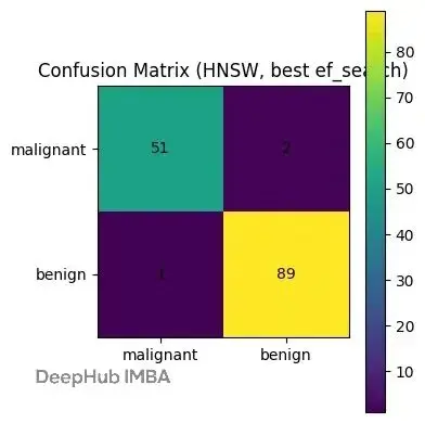
    # Confusion matrix as an operational sanity check (post best ef_search)  
    cm = confusion_matrix(y_test, y_pred)  
    plt.figure(figsize=(4, 4))  
    plt.title("混淆矩陣（HNSW，最佳ef_search）")  
    plt.imshow(cm, interpolation="nearest")  
    plt.colorbar()  
    plt.xticks([0, 1], ["惡性", "良性"])  
    plt.yticks([0, 1], ["惡性", "良性"])  
    for (i, j), val in np.ndenumerate(cm):  
        plt.text(j, i, int(val), ha="center", va="center")  
    plt.tight_layout()  
    plt.show()  

    return {  
        "clf": clf,  
        "train_time_s": train_time,  
        "query_time_s": final_query_time,  
        "acc": final_acc,  
        "f1": final_f1,  
        "sweep": {  
            "ef_search": sweep_ef_search,  
            "times": sweep_times,  
            "acc": sweep_acc,  
            "f1": sweep_f1,  
        },  
    }  

# ======================  
# PHASE 8 — Narrative Glue (Challenge → Insight → Application)  
# ======================  
# Challenge:  
#   Brute-force nearest neighbor search scales poorly; even with modest dimensionality, latency explodes  
#   as data grows. Distance computations become the bottleneck in RAG and real-time ML systems.  
#  
# Insight:  
#   HNSW imposes hierarchy and navigable small-world structure on the vector space. We tune (M, ef_search)  
#   to move along the recall/latency curve. Standardize inputs; consider PCA to enhance neighborhood purity.  
#  
# Application:  
#   Swap KNN brute with HNSW-backed ANN. Cross-validate to pick an operating point. Measure with a  
#   hold-out and visualize ef_search sweeps to institutionalize a *speed-quality contract* with users.  

# ======================  
# PHASE 9 — End-to-end Wrapper  
# ======================  
def run_hnsw_benchmark(  
    test_size: float = 0.25,  
    random_state: int = 42,  
    n_pca: int = 16,  # Try None to keep full dims; 16 often yields stable neighborhoods on this dataset  
) -> None:  
    # 1) Load data  
    X, y, feature_names = load_data()  

    # 2) Quick EDA to connect intuition to modeling choices  
    quick_eda(X, y, feature_names)  

    # 3) Train/Test split (hold-out after CV)  
    X_train, X_test, y_train, y_test = train_test_split(  
        X, y, test_size=test_size, stratify=y, random_state=random_state  
    )  

    # 4) HNSW CV Tuning (on training only)  
    #    We keep the grid small here; practitioners would expand it under time budgets.  
    param_grid = {  
        "M": [12, 16, 32],  
        "ef_construction": [100, 200],  
        "ef_search": [32, 64, 128, 256],  
        "k": [3, 5, 7],  
    }  
    best = hnsw_cv_tuning(  
        X_train, y_train, param_grid, n_splits=5, n_pca=n_pca, random_state=random_state  
    )  

    # 5) Build the final embedding pipeline on train/test with the chosen PCA config  
    X_train_emb, X_test_emb, scaler, pca_model = make_embeddings(  
        X_train, X_test, n_pca=n_pca  
    )  

    # 6) Baseline brute-force kNN, to *quantify* ROI  
    baseline = brute_knn_baseline(  
        X_train_emb, y_train, X_test_emb, y_test, k=best.params["k"]  
    )  
    print("\n=== 基線：暴力k-NN ===")  
    print(  
        f"k={baseline['k']} | 訓練 {baseline['train_time_s']:.4f}s | "  
        f"查詢 {baseline['query_time_s']:.4f}s | "  
        f"準確率={baseline['acc']:.4f} | F1={baseline['f1']:.4f}"  
    )  

    # 7) Final HNSW fit/eval and *visualize the ef_search dial* (the central HNSW idea)  
    sweep = [16, 32, 64, 128, 256, 384]  
    hnsw_out = fit_eval_hnsw_and_visualize(  
        X_train_emb, y_train, X_test_emb, y_test, best.params, sweep  
    )  

    # 8) Final narrative printout to tie back to the essay:  
    print("\n=== 敍述：挑戰→洞察→應用 ===")  
    print(  
        "- 挑戰：暴力k-NN需要掃描所有點併成為系統瓶頸。\n"  
        "- 洞察：HNSW構建分層小世界圖，讓我們權衡搜索廣度（ef_search）\n"  
        "          與準確性和延遲——高效地從粗到細鄰域縮放。\n"  
        "- 應用：我們用交叉驗證調優（M，ef_search，k），選擇高F1操作點，\n"  
        "              並使用ef_search掃描制度化速度-質量合同。"  
    )  

    # 9) Summarize ROI  
    print("\n=== ROI總結（留出測試）===")  
    print(  
        f"暴力kNN：準確率={baseline['acc']:.4f}，F1={baseline['f1']:.4f}，"  
        f"查詢={baseline['query_time_s']:.4f}s"  
    )  
    print(  
        f"HNSW最佳：準確率={hnsw_out['acc']:.4f}，F1={hnsw_out['f1']:.4f}，"  
        f"查詢={hnsw_out['query_time_s']:.4f}s（ef_search={best.params['ef_search']}）"  
    )  
    print(  
        "解釋：如果HNSW以更低的查詢延遲實現可比較或更好的質量，\n"  
        "它驗證了核心工程聲明：*隨着規模增長，更智能的檢索勝過暴力*。"  
    )  

# Entrypoint  
if __name__ == "__main__":  
     run_hnsw_benchmark()

實驗結果：分層確實有效

把數據集想象成一個圖書館，每個向量是一本書。暴力k-NN就像實習生，每次查詢都得翻遍每個書架——靠譜但慢。HNSW是經驗豐富的館員，從頂層開始（粗糙的地圖），直奔正確的區域。

在乳腺癌數據集上，HNSW達到了和暴力搜索相同的測試準確率和F1分數（≈0.979 / 0.983），查詢時間卻只有1/17（≈5毫秒 vs 89毫秒）。這驗證了我們這篇文章的核心論點——非結構化空間中的結構化搜索——從理論變成了實實在在的性能提升。

什麼配置真正起作用

層次結構+小搜索廣度最優

交叉驗證反覆選中了小搜索廣度（ef_search=32）配合適中連接度（M=12）和k=5。參數掃描顯示，把ef_search從16推到384，準確率幾乎不動，延遲卻線性增長。這是因為，一旦定位到正確區域，翻4倍的候選集並不能在這個數據上找到更好的鄰居，純粹是浪費時間。

輕量級特徵處理穩定鄰域

標準化加上PCA降到16維，產生了穩定的鄰域結構和一致的交叉驗證得分，讓HNSW的圖更好導航。不需要花哨的度量學習，基本的數據清洗（縮放+輕度降噪）就足夠暴露HNSW能利用的結構。

和暴力搜索質量持平

混淆矩陣很直白：2個假陰性，1個假陽性。和暴力k-NN完全一個水平。診斷質量沒打折扣，但臨牀系統或下游應用不用再等那麼久。

什麼配置沒起作用

更大的ef_search沒換來準確率

超過32左右，準確率和F1就平了。在這個相對乾淨、分離良好的數據集上，第一批好鄰居已經"夠好"。繼續擴大搜索範圍看起來很好，但實際上像過度管理，只是在燒CPU時間。

更密集的連接（M）也不必要

試過M=12、16、32。圖結構不需要更多鏈接就能找到同樣的答案，對這個任務來説額外的內存和索引時間都是浪費。

暴力搜索在小規模下還行

幾百個樣本的情況下，暴力k-NN的訓練和查詢時間還能接受。重點不是説暴力搜索"不好"，而是HNSW的優勢會隨數據規模增長——即便在小數據集上也能看出這個趨勢。

後續探索方向

大規模試驗（百萬到億級向量）

優勢應該會進一步放大。重點測recall@k vs精確k-NN的差距，P95/P99尾延遲，單向量內存佔用。

度量和嵌入的變體

試試歸一化向量+餘弦距離，用自編碼器替換PCA，或者測領域定製的嵌入。不同幾何結構會改變HNSW的最佳工作點。

壓縮+混合索引

結合HNSW和PQ/OPQ來壓縮內存，量化召回率和延遲的損失。超大語料庫可以評估基於磁盤的HNSW（比如mmap）和熱緩存行為。

在線更新能力

壓測動態插入刪除，看重平衡開銷。流式場景下跟蹤召回率隨時間的漂移。

自適應策略

訓練一個控制器，根據查詢難度（熵、邊距、重排序不確定性）動態設ef_search。簡單查詢少花時間，複雜查詢多給預算。

 === EDA: 基本信息 ===  
樣本數：569，特徵數：30  
類別分佈（0=惡性，1=良性）：{np.int64(0): np.int64(212), np.int64(1): np.int64(357)}  

=== HNSW CV調優：72個配置，5折 ===  
嵌入維度：16（PCA=開啓）  
配置 {'M': 12, 'ef_construction': 100, 'ef_search': 32, 'k': 3} -> F1: 0.9688 | Acc: 0.9601  
配置 {'M': 12, 'ef_construction': 100, 'ef_search': 32, 'k': 5} -> F1: 0.9726 | Acc: 0.9648  
（中間配置結果省略）  
最佳HNSW CV參數：{'M': 12, 'ef_construction': 100, 'ef_search': 32, 'k': 5}（F1=0.9726，Acc=0.9648）  

=== 基線：暴力k-NN ===  
k=5 | 訓練 0.0012s | 查詢 0.0893s | 準確率=0.9790 | F1=0.9834  

=== 最終HNSW（最佳CV參數）===  
參數：{'M': 12, 'ef_construction': 100, 'ef_search': 32, 'k': 5}  
訓練時間：0.0210s | 查詢時間：0.0052s  
測試準確率：0.9790 | F1：0.9834  

分類報告：  
               precision    recall  f1-score   support  
           0     0.9808    0.9623    0.9714        53  
           1     0.9780    0.9889    0.9834        90  
    accuracy                         0.9790       143  

ef_search參數掃描：  
ef_search=16   -> Acc=0.9790, F1=0.9834, QueryTime=0.0043s  
ef_search=32   -> Acc=0.9790, F1=0.9834, QueryTime=0.0053s  
ef_search=64   -> Acc=0.9790, F1=0.9834, QueryTime=0.0070s  
ef_search=128  -> Acc=0.9790, F1=0.9834, QueryTime=0.0107s  
ef_search=256  -> Acc=0.9790, F1=0.9834, QueryTime=0.0231s  
ef_search=384  -> Acc=0.9790, F1=0.9834, QueryTime=0.0223s  

=== ROI總結（留出測試）===  
暴力kNN：準確率=0.9790，F1=0.9834，查詢=0.0893s  
HNSW最佳：準確率=0.9790，F1=0.9834，查詢=0.0052s（ef_search=32）  
結論：HNSW在保持同等質量的前提下，查詢延遲降到原來的1/17，  
 驗證了核心主張：規模增長時，智能檢索完勝暴力掃描。

總結

嵌入向量數量還在指數級增長，HNSW提出了一個簡單事實：智能不是知道所有答案，而是知道先從哪裏找起。

高效AI系統的未來可能更少依賴大模型本身，更多依賴智能檢索。從這個角度看，HNSW不只是個優化技巧，它改變了機器記憶和查詢的底層邏輯。

https://avoid.overfit.cn/post/6e8a792fb0eb4f4ab911cce7f3e98644

作者：Everton Gomede, PhD