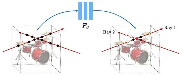
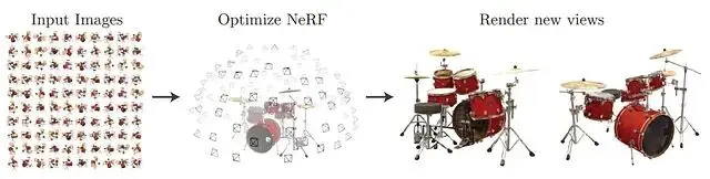
NeRF（Neural Radiance Fields，神經輻射場）的核心思路是用一個全連接網絡表示三維場景。輸入是5D向量空間座標(x, y, z)加上視角方向(θ, φ)，輸出則是該點的顏色和體積密度。訓練的數據則是同一物體從不同角度拍攝的若干張照片。

通常情況下泛化能力是模型的追求目標，需要在大量不同樣本上訓練以避免過擬合。但NeRF恰恰相反，它只在單一場景的多個視角上訓練，刻意讓網絡"過擬合"到這個特定場景，這與傳統神經網絡的訓練邏輯完全相反。

這樣NeRF把網絡訓練成了某個場景的"專家"，這個專家只懂一件事，但懂得很透徹：給它任意一個新視角，它都能告訴你從那個方向看場景是什麼樣子，存儲的不再是一堆圖片，而是場景本身的隱式表示。

基本概念

把5D輸入向量拆開來看：空間位置(x, y, z)和觀察方向(θ, φ)。

顏色（也就是輻射度）同時依賴位置和觀察方向，這很好理解，因為同一個點從不同角度看可能有不同的反光效果。但密度只跟位置有關與觀察方向無關。這裏的假設是材質本身不會因為你換個角度看就變透明或變不透明，這個約束大幅降低了模型複雜度。

用來表示這個映射關係的是一個多層感知機（MLP）而且沒有卷積層，這個MLP被有意過擬合到特定場景。

渲染流程分三步：沿每條光線採樣生成3D點，用網絡預測每個點的顏色和密度，最後用體積渲染把這些顏色累積成二維圖像。

訓練時用梯度下降最小化渲染圖像與真實圖像之間的差距。不過直接訓練效果不好原始5D輸入需要經過位置編碼轉換才能讓網絡更好地捕捉高頻細節。

傳統體素表示需要顯式存儲整個場景佔用空間巨大。NeRF則把場景信息壓縮在網絡參數裏，最終模型可以比原始圖片集小很多。這是NeRF的一個關鍵優勢。

相關工作

NeRF出現之前，神經場景表示一直比不過體素、三角網格這些離散表示方法。

早期也有人用網絡把位置座標映射到距離函數或佔用場，但只能處理ShapeNet這類合成3D數據。

arxiv:1912.07372 用3D佔用場做隱式表示提出了可微渲染公式。arxiv:1906.01618的方法在每個3D點輸出特徵向量和顏色用循環神經網絡沿光線移動來檢測表面,但這些方法生成的表面往往過於平滑。

如果視角採樣足夠密集，光場插值技術就能生成新視角。但視角稀疏時必須用表示方法,體積方法能生成真實感強的圖像但分辨率上不去。

場景表示機制

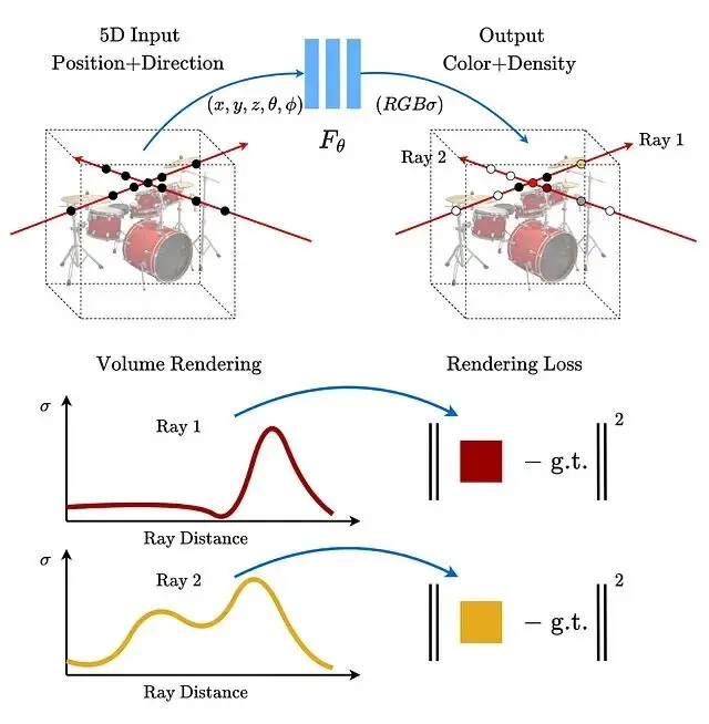
輸入是位置 x = (x, y, z) 和觀察方向 d = (θ, φ)，輸出是顏色 c = (r, g, b) 和密度 σ。整個5D映射用MLP來近似。

優化目標是網絡權重 Θ。密度被假設為多視角一致的，顏色則同時取決於位置和觀察方向。

網絡結構上先用8個全連接層處理空間位置，輸出密度σ和一個256維特徵向量。這個特徵再和觀察方向拼接，再經過一個全連接層得到顏色。

體積渲染

光線參數化如下：

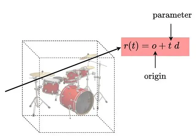
密度σ描述的是某點對光線的阻擋程度，可以理解為吸收概率。更嚴格地説它是光線在該點終止的微分概率。根據這個定義，光線從t傳播到tₙ的透射概率可以表示為：

σ和T之間的關係可以畫圖來理解：

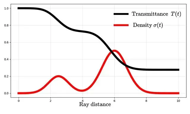
密度升高時透射率下降。一旦透射率降到零，後面的東西就完全被遮住了，也就是看不見了。

光線的期望顏色C(r)定義如下，沿光線從近到遠積分：

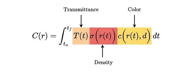
問題在於c和σ都來自神經網絡這個積分沒有解析解。

實際計算時用數值積分，採用分層採樣策略——把積分範圍分成N個區間，每個區間均勻隨機抽一個點。

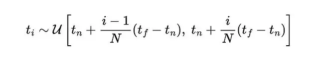
分層採樣保證MLP在整個優化過程中都能在連續位置上被評估。採樣點通過求積公式計算C(t)這個公式選擇上考慮了可微性。跟純隨機採樣比方差更低。

Tᵢ是光線存活到第i個區間之前的概率。那光線在第i個區間內終止的概率呢？可以用密度來算：

σ越大這個概率越趨近於零，再往下推導：

光線顏色可以寫成：

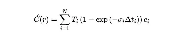
其中：

位置編碼

直接拿5D座標訓練MLP，高頻細節渲染不出來。因為深度網絡天生偏好學習低頻信號，解決辦法是用高頻函數把輸入映射到更高維空間。

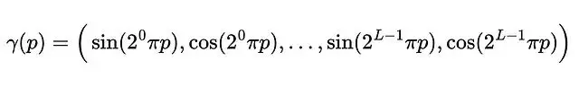
γ對每個座標分別應用，是個確定性函數沒有可學習參數。p歸一化到[-1,+1]。L=4時的編碼可視化：

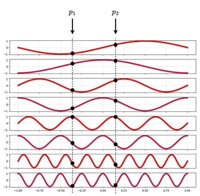
L=4時的位置編碼示意

編碼用的是不同頻率的正弦函數。Transformer裏也用類似的位置編碼但目的不同——Transformer是為了讓模型感知token順序，NeRF是為了注入高頻信息。

分層採樣

均勻採樣的問題在於大量計算浪費在空曠區域。分層採樣的思路是訓練兩個網絡，一個粗糙一個精細。

先用粗糙網絡採樣評估一批點，再根據結果用逆變換採樣在重要區域加密採樣。精細網絡用兩組樣本一起計算最終顏色。粗糙網絡的顏色可以寫成採樣顏色的加權和。

實現

每個場景單獨訓練一個網絡，只需要RGB圖像作為訓練數據。每次迭代從所有像素裏採樣一批光線，損失函數是粗糙和精細網絡預測值與真值之間的均方誤差。

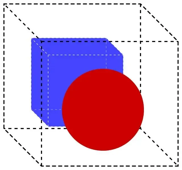
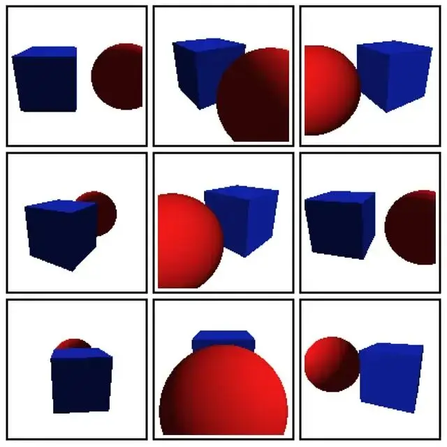
接下來從零實現NeRF架構，在一個包含藍色立方體和紅色球體的簡單數據集上訓練。

數據集生成代碼不在本文範圍內——只涉及基礎幾何變換沒有NeRF特有的概念。

數據集裏的一些渲染圖像。相機矩陣和座標也存在了JSON文件裏。

先導入必要的庫：

 import os, json, math  
 import numpy as np  
 from PIL import Image  
 import torch  
 import torch.nn as nn  
 import torch.nn.functional as F

位置編碼函數：

 def positional_encoding(x, L):  
     freqs = (2.0 ** torch.arange(L, device=x.device)) * math.pi # Define the frequencies  
     xb = x[..., None, :] * freqs[:, None] # Multiply by the frequencies  
     xb = xb.reshape(*x.shape[:-1], L * 3) # Flatten the (x,y,z) coordinates  
     return torch.cat([torch.sin(xb), torch.cos(xb)], dim=-1)

根據相機參數生成光線：

 def get_rays(H, W, camera_angle_x, c2w, device):  
    # assume the pinhole camera model  
    fx = 0.5 * W / math.tan(0.5 * camera_angle_x) # calculate the focal lengths (assume fx=fy)  

    # principal point of the camera or the optical center of the image.   
    cx = (W - 1) * 0.5   
    cy = (H - 1) * 0.5  

    i, j = torch.meshgrid(torch.arange(W, device=device),  
                          torch.arange(H, device=device), indexing="xy")  
    i, j = i.float(), j.float()  
      
    # convert pixels to normalized camera-plane coordinates  
    x = (i - cx) / fx  
    y = -(j - cy) / fx  
    z = -torch.ones_like(x)  

    # pack into 3D directions and normalize  
    dirs = torch.stack([x, y, z], dim=-1)  
    dirs = dirs / torch.norm(dirs, dim=-1, keepdim=True)  
      
    # rotate rays into world coordinates using pose matrix  
    R, t = c2w[:3, :3], c2w[:3, 3]  
    rd = dirs @ R.T  
    ro = t.expand_as(rd)  
     return ro, rd

NeRF網絡結構：

 class NeRF(nn.Module):  
    def __init__(self, L_pos=10, L_dir=4, hidden=256):  
        super().__init__()  
        # original vector is concatented with the fourier features  
        in_pos = 3 + 2 * L_pos * 3  
        in_dir = 3 + 2 * L_dir * 3  

        self.fc1 = nn.Linear(in_pos, hidden)  
        self.fc2 = nn.Linear(hidden, hidden)  
        self.fc3 = nn.Linear(hidden, hidden)  
        self.fc4 = nn.Linear(hidden, hidden)  
        self.fc5 = nn.Linear(hidden + in_pos, hidden)  
        self.fc6 = nn.Linear(hidden, hidden)  
        self.fc7 = nn.Linear(hidden, hidden)  
        self.fc8 = nn.Linear(hidden, hidden)  

        self.sigma = nn.Linear(hidden, 1)  
        self.feat = nn.Linear(hidden, hidden)  

        self.rgb1 = nn.Linear(hidden + in_dir, 128)  
        self.rgb2 = nn.Linear(128, 3)  

        self.L_pos, self.L_dir = L_pos, L_dir  

    def forward(self, x, d):  
        x_enc = torch.cat([x, positional_encoding(x, self.L_pos)], dim=-1)  
        d_enc = torch.cat([d, positional_encoding(d, self.L_dir)], dim=-1)  

        h = F.relu(self.fc1(x_enc))  
        h = F.relu(self.fc2(h))  
        h = F.relu(self.fc3(h))  
        h = F.relu(self.fc4(h))  
        h = torch.cat([h, x_enc], dim=-1) # skip connection  
        h = F.relu(self.fc5(h))  
        h = F.relu(self.fc6(h))  
        h = F.relu(self.fc7(h))  
        h = F.relu(self.fc8(h))  

        sigma = F.relu(self.sigma(h)) # density is calculated using positional information  
        feat = self.feat(h)  

        h = torch.cat([feat, d_enc], dim=-1) # add directional information for color  
        h = F.relu(self.rgb1(h))  
        rgb = torch.sigmoid(self.rgb2(h))  
         return rgb, sigma

渲染函數，這個是整個流程的核心：

 def render_rays(model, ro, rd, near=2.0, far=6.0, N=64):  
    # sample along the ray  
    t = torch.linspace(near, far, N, device=ro.device)  
    pts = ro[:, None, :] + rd[:, None, :] * t[None, :, None] # r = o + td  
      
    # attach view directions to each sample  
    # each point knows where the ray comes from  
    dirs = rd[:, None, :].expand_as(pts)  
      
    # query NeRF at each point and reshape  
    rgb, sigma = model(pts.reshape(-1,3), dirs.reshape(-1,3))  
    rgb = rgb.reshape(ro.shape[0], N, 3)  
    sigma = sigma.reshape(ro.shape[0], N)  

    # compute the distance between the samples  
    delta = t[1:] - t[:-1]  
    delta = torch.cat([delta, torch.tensor([1e10], device=ro.device)])  

    # convert density into opacity  
    alpha = 1 - torch.exp(-sigma * delta)  
    # compute transmittance along the ray  
    T = torch.cumprod(torch.cat([torch.ones((ro.shape[0],1), device=ro.device),  
                                 1 - alpha + 1e-10], dim=-1), dim=-1)[:, :-1]  

    weights = T * alpha  
     return (weights[...,None] * rgb).sum(dim=1) # accumulate the colors

訓練循環：

 device = "cuda" if torch.cuda.is_available() else "cpu"  
images, c2ws, H, W, fov = load_dataset("nerf_synth_cube_sphere")  
images, c2ws = images.to(device), c2ws.to(device)  

model = NeRF().to(device)  
opt = torch.optim.Adam(model.parameters(), lr=5e-4)  

loss_hist, psnr_hist, iters = [], [], []  

for it in range(1, 5001):  
    idx = torch.randint(0, images.shape[0], (1,)).item()  
    ro, rd = get_rays(H, W, fov, c2ws[idx], device)  
    gt = images[idx].reshape(-1,3)  

    sel = torch.randint(0, ro.numel()//3, (2048,), device=device)  
    pred = render_rays(model, ro.reshape(-1,3)[sel], rd.reshape(-1,3)[sel])  
      
    # for simplicity, we will only implement the coarse sampling.   
    loss = F.mse_loss(pred, gt[sel])  

    opt.zero_grad()  
    loss.backward()  
    opt.step()  

    if it % 200 == 0:  
        psnr = -10 * torch.log10(loss).item()  
        loss_hist.append(loss.item())  
        psnr_hist.append(psnr)  
        iters.append(it)  
        print(f"Iter {it} | Loss {loss.item():.6f} | PSNR {psnr:.2f} dB")  

torch.save(model.state_dict(), "nerf_cube_sphere_coarse.pth")  

# ---- Plots ----  
plt.figure()  
plt.plot(iters, loss_hist, color='red', lw=5)  
plt.title("Training Loss")  
plt.show()  

plt.figure()  
plt.plot(iters, psnr_hist, color='black', lw=5)  
plt.title("Training PSNR")  
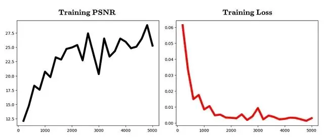
 plt.show()

迭代次數與PSNR、損失值的變化曲線：

模型訓練完成下一步是生成新視角。

look_at

函數用於從指定相機位置構建位姿矩陣：

 def look_at(eye):  
    eye = torch.tensor(eye, dtype=torch.float32) # where the camera is  
    target = torch.tensor([0.0, 0.0, 0.0])  
    up = torch.tensor([0,1,0], dtype=torch.float32) # which direction is "up" in the world  

    f = (target - eye); f /= torch.norm(f) # forward direction of the camera  
    r = torch.cross(f, up); r /= torch.norm(r) # right direction. use cross product between f and up  
    u = torch.cross(r, f) # true camera up direction  

    c2w = torch.eye(4)  
    c2w[:3,0], c2w[:3,1], c2w[:3,2], c2w[:3,3] = r, u, -f, eye  
     return c2w

推理代碼：

 device = "cuda" if torch.cuda.is_available() else "cpu"  

with open("nerf_synth_cube_sphere/transforms.json") as f:  
    meta = json.load(f)  

H, W, fov = meta["h"], meta["w"], meta["camera_angle_x"]  

model = NeRF().to(device)  
model.load_state_dict(torch.load("nerf_cube_sphere_coarse.pth", map_location=device))  
model.eval()  

os.makedirs("novel_views", exist_ok=True)  

for i in range(120):  
    angle = 2 * math.pi * i / 120  
    eye = [4 * math.cos(angle), 1.0, 4 * math.sin(angle)]  
    c2w = look_at(eye).to(device)  

    with torch.no_grad():  
        ro, rd = get_rays(H, W, fov, c2w, device)  
        rgb = render_rays(model, ro.reshape(-1,3), rd.reshape(-1,3))  

    img = rgb.reshape(H, W, 3).clamp(0,1).cpu().numpy()  
    Image.fromarray((img*255).astype(np.uint8)).save(f"novel_views/view_{i:03d}.png")  

     print("Rendered view", i)

新視角渲染結果（訓練集中沒有這些角度）：

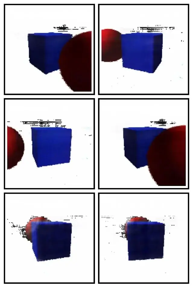
圖中的偽影——椒鹽噪聲、條紋、浮動的亮點——來自空曠區域的密度估計誤差。只用粗糙模型、不做精細採樣的情況下這些問題會更明顯。另外場景裏大片空白區域也是個麻煩，模型不得不花大量計算去探索這些沒什麼內容的地方。

再看看深度圖：

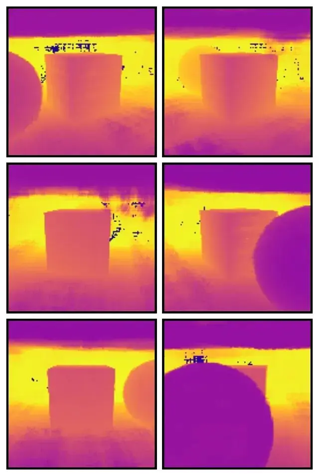
立方體的平面捕捉得相當準確沒有幽靈表面。空曠區域有些斑點噪聲説明雖然空白區域整體學得還行，但稀疏性還是帶來了一些小誤差。

參考文獻

Mildenhall, B., Srinivasan, P. P., Gharbi, M., Tancik, M., Barron, J. T., Simonyan, K., Abbeel, P., & Malik, J. (2020). NeRF: Representing scenes as neural radiance fields for view synthesis.

https://avoid.overfit.cn/post/4a1b21ea7d754b81b875928c95a45856

作者：Kavishka Abeywardana