Transformer的"二次方注意力瓶頸"的問題是老生常談了。這個瓶頸到底卡在哪實際工程裏怎麼繞過去？本文從一個具體問題出發，介紹Mosaic這套多軸注意力分片方案的設計思路。

注意力的內存困境

注意力機制的計算公式：

 Attention(Q, K, V) = softmax(QKᵀ / √d) × V

問題出在 QKᵀ 這個矩陣上，它的形狀是

(序列長度 × 序列長度)

。

拿150,000個token的序列算一下：

 Memory = 150,000² × 4 bytes = 90 billion bytes ≈ 84 GB

這只是注意力權重本身的開銷，而且還是單層、單頭。A100的顯存上限是80GB，放不下就是放不下。

現有方案的侷限

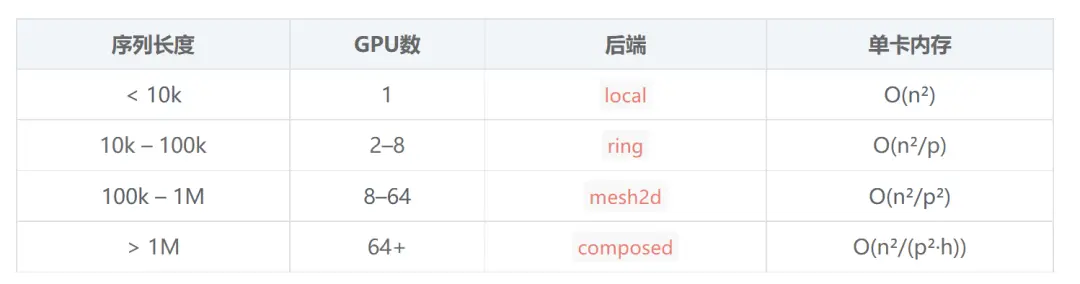
FlashAttention 它通過分塊計算，不需要把完整的注意力矩陣實例化出來，內存複雜度從O(n²)降到O(n)。單卡場景下效果很好，但問題是整個序列還是得塞進同一張GPU。

Ring Attention 換了個思路：把序列切片分到多張GPU上，每張卡持有一部分Q，K和V在GPU之間像傳令牌一樣輪轉，一維序列處理起來是很不錯的。

但是多維怎麼辦？

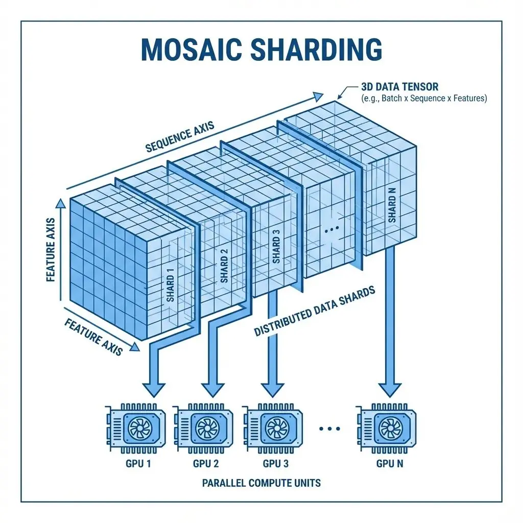
比如處理表格數據的Transformer，輸入張量形狀是

(batch, rows, features, embed)

。模型需要在不同維度上做注意力：features維度只有5個token，rows維度卻有150,000個。前者單卡輕鬆搞定，後者則必須分片。

現有的庫都沒法乾淨地處理這種多軸場景。手寫的話，每個軸要單獨寫分片邏輯，進程組管理、張量reshape全得自己來。代碼會變得很髒。

Mosaic的設計

Mosaic本質上是個協調層，負責把不同的注意力軸路由到合適的計算後端：

 import mosaic

# Small axis: run locally
feature_attn = mosaic.MultiAxisAttention(  
    embed_dim=96,   
    num_heads=4,  
    attention_axis=2,    # features dimension
    backend="local"      # no communication needed
)

# Large axis: shard across GPUs
row_attn = mosaic.MultiAxisAttention(  
    embed_dim=96,   
    num_heads=4,  
    attention_axis=1,    # rows dimension
    backend="ring"       # ring attention across GPUs
 )

底層Mosaic會自動處理軸的置換、QKV投影前的reshape、後端分發、以及計算完成後張量形狀的還原。模型代碼保持清晰，分佈式的複雜性被封裝掉了。

Ring Attention的工作機制

核心思想其實很直接：不需要同時持有全部的K和V。可以分批計算注意力分數，逐步累積，最後再做歸一化。

比如説4張GPU的情況下流程是這樣的：

 Initial state:  
  GPU 0: Q₀, K₀, V₀  
  GPU 1: Q₁, K₁, V₁    
  GPU 2: Q₂, K₂, V₂  
  GPU 3: Q₃, K₃, V₃

Step 1: Each GPU computes attention with its local K, V  
  GPU 0: score₀₀ = Q₀ @ K₀ᵀ  
  ...

Step 2: Pass K, V to the next GPU in the ring  
  GPU 0 receives K₃, V₃ from GPU 3  
  GPU 0 sends K₀, V₀ to GPU 1  
    
Step 3: Compute attention with received K, V  
  GPU 0: score₀₃ = Q₀ @ K₃ᵀ  
  Accumulate with score₀₀

Repeat for all chunks...

 Final: Each GPU has complete attention output for its Q chunk

單卡內存佔用變成O(n²/p)，p是GPU數量。8張卡的話內存需求直接砍到1/8。150k序列從84GB降到約10GB每卡。

Mesh2D：更激進的分片

序列特別長的時候Ring Attention的線性分片可能還不夠，這時候可以用Mesh2D把Q和K都切分了：

 4 GPUs arranged in 2×2 mesh:

          K₀    K₁  
       ┌──────┬──────┐  
  Q₀   │GPU 0 │GPU 1 │  
       ├──────┼──────┤  
  Q₁   │GPU 2 │GPU 3 │  
       └──────┴──────┘  
         
 Each GPU computes one tile of QKᵀ

內存複雜度降到O(n²/p²)。64張卡組成8×8網格時，每卡內存需求下降64倍。

 attn=mosaic.MultiAxisAttention(  
     embed_dim=128,   
     num_heads=8,  
     attention_axis=1,  
     backend="mesh2d",  
     mesh_shape=(8, 8)  
 )

感知集羣拓撲的組合策略

在實際部署環境裏，不同GPU之間的通信帶寬差異很大。節點內GPU走NVLink能到900 GB/s，跨節點通過InfiniBand通常只有200 GB/s左右。

ComposedAttention

就是針對這種拓撲特徵設計的：

 # 4 nodes × 8 GPUs = 32 total
 composed = mosaic.ComposedAttention(  
     mesh_shape=(4, 8),       # (nodes, gpus_per_node)
     head_parallel=True,      # Split heads across nodes (slow link)
     seq_parallel="ring"      # Ring within nodes (fast link)
 )

需要更精細控制的話，可以用

HierarchicalAttention

：

 hier = mosaic.HierarchicalAttention(  
     intra_node_size=8,  
     intra_node_strategy="local",   # Compute locally within node
     inter_node_strategy="ring"     # Ring between node leaders
 )

重通信走快鏈路輕通信才跨節點。

實現細節

整個庫大約800行Python，核心代碼如下：

 class MultiAxisAttention(nn.Module):  
    def forward(self, x):  
        # 1. Move attention axis to seq position
        x, inv_perm = self._permute_to_seq(x)  
          
        # 2. Flatten batch dims, project QKV
        x = x.view(-1, seq_len, embed_dim)  
        qkv = self.qkv_proj(x).view(batch, seq, 3, heads, head_dim)  
        q, k, v = qkv.permute(2, 0, 3, 1, 4).unbind(0)  
          
        # 3. Dispatch to backend
        out = self._attn_fn(q, k, v)  # local, ring, or mesh2d
          
        # 4. Project output, restore shape
        out = self.out_proj(out.transpose(1, 2).reshape(...))  
         return out.permute(inv_perm)

後端封裝了現有的成熟實現：

local

後端調用

F.scaled_dot_product_attention

（也就是FlashAttention），

ring

後端用ring-flash-attn庫的

ring_flash_attn_func

，

mesh2d

是自定義的all-gather加SDPA，所有的底層都跑的是FlashAttention內核。

所有後端統一用FlashAttention的融合GEMM+softmax實現。後端函數在初始化時就綁定好，前向傳播不做分支判斷。張量操作儘量用

x.view()

而不是

x.reshape()

，保持內存連續性。集合通信的目標張量預分配好，避免

torch.cat

的開銷。模塊級別做導入不在每次前向傳播時產生import開銷。

快速上手

安裝：

 pip install git+https://github.com/stprnvsh/mosaic.git
 
 # With ring attention support
 pip install flash-attn ring-flash-attn

單節點啓動：

 torchrun --nproc_per_node=4 train.py

多節點的話：

 # Node 0
 torchrun --nnodes=2 --nproc_per_node=8 --node_rank=0 \  
          --master_addr=192.168.1.100 --master_port=29500 train.py
 
 # Node 1
 torchrun --nnodes=2 --nproc_per_node=8 --node_rank=1 \  
          --master_addr=192.168.1.100 --master_port=29500 train.py

訓練腳本示例：

 import mosaic  
import torch.distributed as dist

dist.init_process_group("nccl")  
ctx = mosaic.init(sp_size=dist.get_world_size())

model = MyModel().to(ctx.device)

# Data is pre-sharded: each GPU has seq_total / world_size tokens
x_local = load_my_shard()  
 out = model(x_local)  # Communication handled by Mosaic

總結

最後，Mosaic不會自動並行化模型（這個用nnScaler），不管數據並行（PyTorch DDP/FSDP的事），也不處理模型分片（交給FSDP或Megatron）。

Mosaic專注於一件事：多軸注意力的分片路由，這套方案最初是給 nanoTabPFN 做的，一個表格數據Transformer。

這個模型要同時在rows（150k個）和features（5個）兩個維度做注意力。標準Ring Attention對維度語義沒有感知，它只認序列這個概念，分不清rows和features的區別。

所以Mosaic需求很明確：小軸本地算，大軸分佈式算，軸的路由邏輯不能侵入模型代碼，有興趣的可以試試。

https://avoid.overfit.cn/post/791e0f30540e4d289a43d01d383e8ab2

作者：Pranav Sateesh