
🤵♂️ 個人主頁:@艾派森的個人主頁
✍🏻作者簡介:Python學習者
🐋 希望大家多多支持,我們一起進步!😄
如果文章對你有幫助的話,
歡迎評論 💬點贊👍🏻 收藏 📂加關注+
目錄
1.項目背景
2.數據集介紹
3.技術工具
4.實驗過程
4.1導入數據
4.2數據預處理
4.3模型編譯
4.4模型訓練
4.5模型評估
4.6結果可視化
源代碼
1.項目背景
近年來,隨着醫學影像數據的快速增長和人工智能技術的迅猛發展,深度學習在輔助醫療診斷領域展現出巨大的應用潛力。腦腫瘤作為一種常見的顱內病變,其早期發現和精準分類對臨牀治療至關重要。傳統的診斷方法主要依賴放射科醫生人工分析核磁共振圖像,這不僅耗時耗力,而且容易受到主觀經驗的影響。雖然基於卷積神經網絡的模型在醫學影像分析中取得了顯著進展,但其局部感知特性在處理需要全局上下文信息的複雜病灶時仍存在一定侷限。在此背景下,Google Research於2020年提出的Vision Transformer模型通過自注意力機制實現了對圖像全局特徵的捕捉,為醫學圖像分析提供了新的技術路徑。本項目旨在探索ViT模型在腦腫瘤MRI圖像檢測任務中的適用性,通過構建端到端的智能診斷系統,實現對腦膠質瘤、腦膜瘤等常見腫瘤的自動識別與分類,為提升醫療診斷效率與準確性提供新的技術支撐。
2.數據集介紹
腦腫瘤是全球面臨的嚴峻健康挑戰,早期發現對有效治療至關重要。MRI(磁共振成像)是診斷腦腫瘤最常用的技術之一,因為它能夠提供腦部軟組織的詳細圖像。
該數據集包含分為兩類的 MRI 圖像:
- (是)對於腦腫瘤圖像
- (否)對於沒有腦腫瘤的圖像
該數據集專為二元分類任務而設計,可用於訓練和評估機器學習或深度學習模型,特別是卷積神經網絡(CNN)。
圖像收集自公開的醫學影像庫和開放的研究出版物,可用於教育和研究。數據集已整理到單獨的文件夾中,方便初學者和研究人員直接用於模型訓練。
該數據集的主要目的是為希望將計算機視覺技術應用於醫學成像領域的學生、研究人員和從業人員提供易於入門且隨時可用的資源。項目範圍涵蓋從簡單的 CNN 分類到更高級的應用,例如遷移學習和模型可解釋性(例如 Grad-CAM 可視化)。
3.技術工具
Python版本:3.9
代碼編輯器:jupyter notebook
4.實驗過程
4.1導入數據
首先導入本次實驗用到的第三方庫並加載數據集
import os
import cv2
import warnings
import timm
import torch
import copy
import types
import torch.nn as nn
import torch.optim as optim
import pandas as pd
import numpy as np
import albumentations as A
import matplotlib.pyplot as plt
import seaborn as sns
import plotly.express as px

from tqdm import tqdm
from PIL import Image
from collections import defaultdict
from sklearn.model_selection import StratifiedShuffleSplit
from sklearn.metrics import confusion_matrix, classification_report, roc_curve, auc
from albumentations.pytorch import ToTensorV2
from torch.utils.data import Dataset, DataLoader
from torch.optim.lr_scheduler import CosineAnnealingLR

sns.set_style("darkgrid")
warnings.filterwarnings('ignore')
DATA_DIR = './brain_tumor_dataset'
classes = [folder for folder in os.listdir(DATA_DIR) if os.path.isdir(os.path.join(DATA_DIR, folder))]查看數據信息
data = []
for cls in classes:
class_path = os.path.join(DATA_DIR, cls)
for filename in os.listdir(class_path):
filepath = os.path.join(class_path, filename)
data.append({'filepath': filepath, 'label': cls})
df = pd.DataFrame(data)
df = df.sample(frac=1).reset_index(drop=True)
display(df.head())
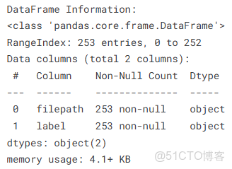
print("\n\nDataFrame Information:")
df.info()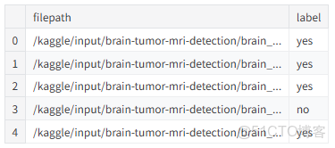
查看腫瘤和非腫瘤圖片
plt.figure(figsize=(15, 8))
n_samples = 5
yes_samples = df[df['label'] == 'yes'].sample(n_samples)
for i, row in enumerate(yes_samples.iterrows()):
filepath = row[1]['filepath']
img = cv2.imread(filepath)
img = cv2.cvtColor(img, cv2.COLOR_BGR2RGB)
plt.subplot(2, n_samples, i + 1)
plt.imshow(img)
plt.title(f"Tumor Detected\n(Class: yes)")
plt.axis('off')
no_samples = df[df['label'] == 'no'].sample(n_samples)
for i, row in enumerate(no_samples.iterrows()):
filepath = row[1]['filepath']
img = cv2.imread(filepath)
img = cv2.cvtColor(img, cv2.COLOR_BGR2RGB)
plt.subplot(2, n_samples, n_samples + i + 1)
plt.imshow(img)
plt.title(f"No Tumor\n(Class: no)")
plt.axis('off')
plt.tight_layout()
plt.show()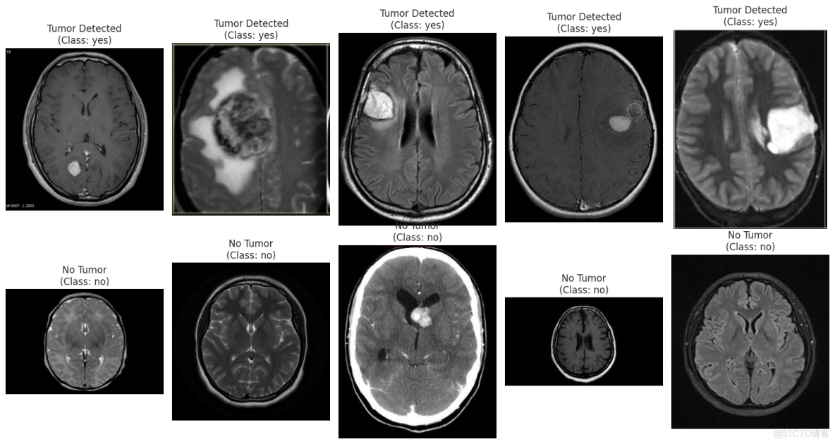
4.2數據預處理
查看數據類別分佈
class_counts = df['label'].value_counts()
fig_pie = px.pie(
names=class_counts.index,
values=class_counts.values,
title='Class Distribution of Brain Tumor MRI',
color_discrete_sequence=px.colors.qualitative.Pastel
)
fig_pie.update_traces(textposition='inside', textinfo='percent+label')
fig_pie.show()
plt.figure(figsize=(8, 6))
sns.countplot(x='label', data=df, palette='viridis')
plt.title('Count of Images per Class')
plt.xlabel('Class Label')
plt.ylabel('Number of Images')
plt.show()
print(class_counts)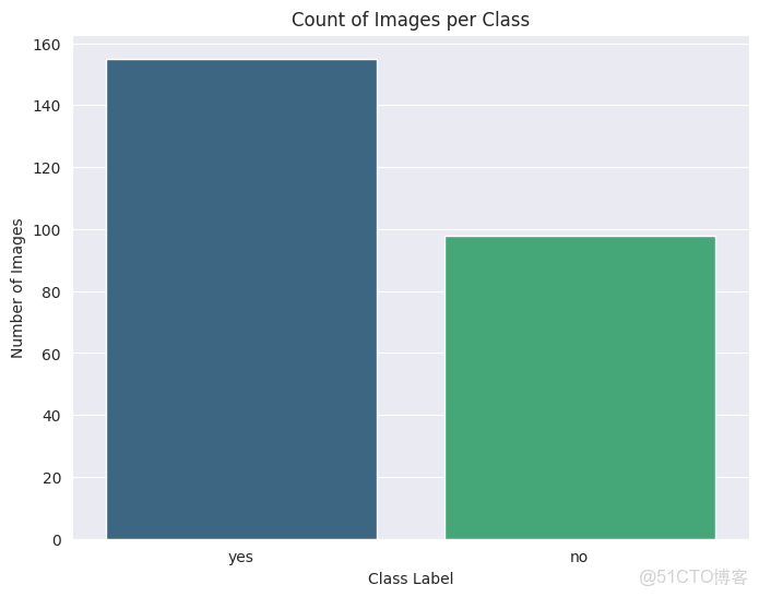
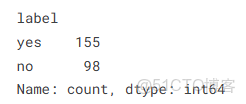
可以看出這些類別是不平衡的。
圖像尺寸分析(可視化高度和寬度的分佈)
heights = []
widths = []
for filepath in tqdm(df['filepath'], desc="Reading image dimensions"):
try:
img = cv2.imread(filepath)
h, w, _ = img.shape
heights.append(h)
widths.append(w)
except Exception as e:
print(f"Could not read {filepath}: {e}")
df['height'] = heights
df['width'] = widths
plt.figure(figsize=(14, 6))
plt.subplot(1, 2, 1)
sns.histplot(df['height'], kde=True, color='skyblue').set_title('Distribution of Image Heights')
plt.subplot(1, 2, 2)
sns.histplot(df['width'], kde=True, color='salmon').set_title('Distribution of Image Widths')
plt.show()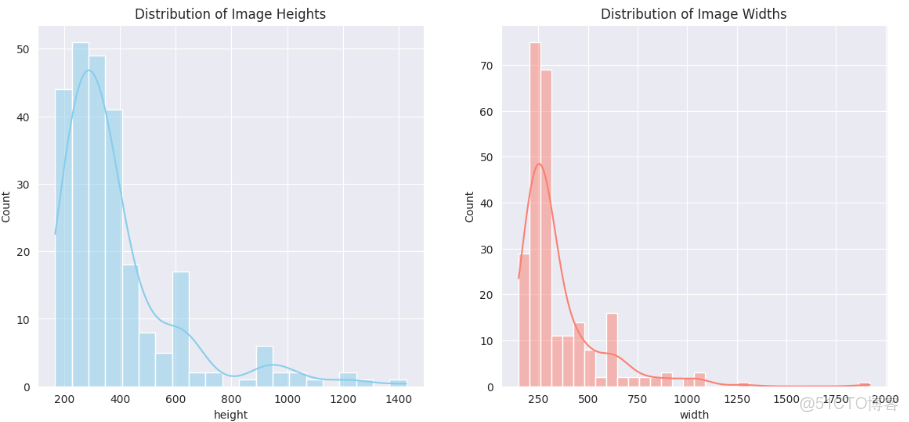
IMG_SIZE = 224
avg_yes = np.zeros((IMG_SIZE, IMG_SIZE, 3), np.float64)
avg_no = np.zeros((IMG_SIZE, IMG_SIZE, 3), np.float64)
count_yes = len(df[df['label'] == 'yes'])
count_no = len(df[df['label'] == 'no'])
for filepath in tqdm(df[df['label'] == 'yes']['filepath'], desc="Averaging 'yes' images"):
img = cv2.imread(filepath)
img = cv2.cvtColor(img, cv2.COLOR_BGR2RGB)
img = cv2.resize(img, (IMG_SIZE, IMG_SIZE))
avg_yes += img / count_yes
for filepath in tqdm(df[df['label'] == 'no']['filepath'], desc="Averaging 'no' images"):
img = cv2.imread(filepath)
img = cv2.cvtColor(img, cv2.COLOR_BGR2RGB)
img = cv2.resize(img, (IMG_SIZE, IMG_SIZE))
avg_no += img / count_no
avg_yes_img = np.array(np.round(avg_yes), dtype=np.uint8)
avg_no_img = np.array(np.round(avg_no), dtype=np.uint8)
print("\nDisplaying the 'average' brain MRI for each class:")
plt.figure(figsize=(12, 6))
plt.subplot(1, 2, 1)
plt.imshow(avg_no_img)
plt.title('Average Non-Tumorous Brain')
plt.axis('off')
plt.subplot(1, 2, 2)
plt.imshow(avg_yes_img)
plt.title('Average Tumorous Brain')
plt.axis('off')
plt.suptitle('Mean Image Representation by Class', fontsize=16)
plt.show()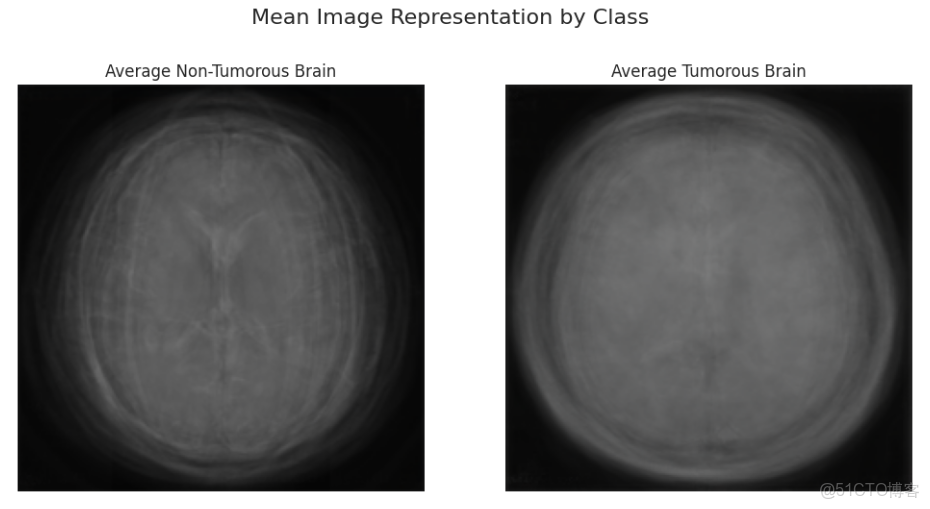
平均的腫瘤腦圖像似乎有一個稍亮、模糊、密集、更明確的中心區域,暗示了該數據集中腫瘤的共同位置或外觀。這表明空間信息是我們的模型學習的一個非常強烈的信號。另一方面,非腫瘤腦圖像更加透明和清晰。
IMG_SIZE = 224
BATCH_SIZE = 32
MEAN = [0.485, 0.456, 0.406]
STD = [0.229, 0.224, 0.225]
splitter = StratifiedShuffleSplit(n_splits=1, test_size=0.2, random_state=666)
for train_index, val_index in splitter.split(df, df['label']):
train_df = df.iloc[train_index]
val_df = df.iloc[val_index]
train_df = train_df.reset_index(drop=True)
val_df = val_df.reset_index(drop=True)
print("Training data info:")
print(train_df['label'].value_counts(normalize=True))
print("\nValidation data info:")
print(val_df['label'].value_counts(normalize=True))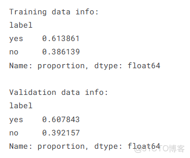
train_transforms = A.Compose([
A.Resize(IMG_SIZE, IMG_SIZE),
A.HorizontalFlip(p=0.5),
A.Rotate(limit=20, p=0.7),
A.RandomBrightnessContrast(brightness_limit=0.2, contrast_limit=0.2, p=0.7),
A.ElasticTransform(alpha=1, sigma=50, alpha_affine=50, p=0.5),
A.CoarseDropout(max_holes=8, max_height=IMG_SIZE//8, max_width=IMG_SIZE//8,
min_holes=1, fill_value=0, p=0.5),
A.Normalize(mean=MEAN, std=STD),
ToTensorV2()
])
val_transforms = A.Compose([
A.Resize(IMG_SIZE, IMG_SIZE),
A.Normalize(mean=MEAN, std=STD),
ToTensorV2()
])創建自定義PyTorch數據集
class BrainMRIDataset(Dataset):
def __init__(self, df, transforms=None):
self.df = df
self.transforms = transforms
self.labels = self.df['label'].map({'yes': 1, 'no': 0}).values
def __len__(self):
return len(self.df)
def __getitem__(self, idx):
filepath = self.df.loc[idx, 'filepath']
label = self.labels[idx]
image = cv2.imread(filepath)
image = cv2.cvtColor(image, cv2.COLOR_BGR2RGB)
if self.transforms:
transformed = self.transforms(image=image)
image = transformed['image']
return image, torch.tensor(label, dtype=torch.float32)temp_train_dataset = BrainMRIDataset(train_df, transforms=train_transforms)
print("Visualizing some of the applied augmentations on a single training image:")
n_images = 8
original_image, _ = temp_train_dataset[0]
viz_transforms = A.Compose([t for t in temp_train_dataset.transforms if not isinstance(t, (A.Normalize, ToTensorV2))])
raw_img = cv2.imread(temp_train_dataset.df.loc[0, 'filepath'])
raw_img = cv2.cvtColor(raw_img, cv2.COLOR_BGR2RGB)
plt.figure(figsize=(16, 8))
plt.subplot(2, (n_images + 1) // 2, 1)
plt.imshow(raw_img)
plt.title("Original Image")
plt.axis('off')
for i in range(1, n_images):
augmented = viz_transforms(image=raw_img)['image']
plt.subplot(2, (n_images + 1) // 2, i + 1)
plt.imshow(augmented)
plt.title(f"Augmented {i}")
plt.axis('off')
plt.tight_layout()
plt.show()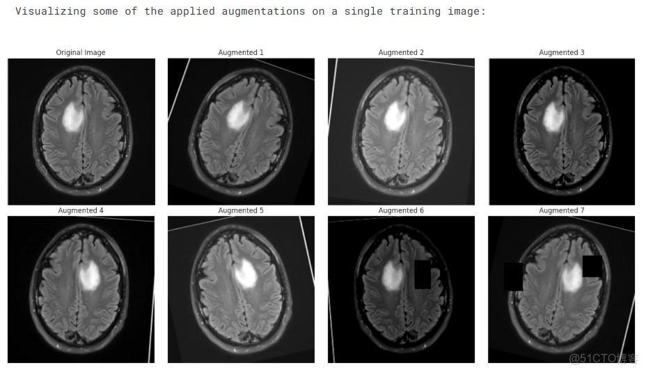
創建DataLoaders
train_dataset = BrainMRIDataset(train_df, transforms=train_transforms)
val_dataset = BrainMRIDataset(val_df, transforms=val_transforms)
train_loader = DataLoader(train_dataset, batch_size=BATCH_SIZE, shuffle=True, num_workers=2)
val_loader = DataLoader(val_dataset, batch_size=BATCH_SIZE, shuffle=False, num_workers=2)
print(f"\nNumber of training batches: {len(train_loader)}")
print(f"Number of validation batches: {len(val_loader)}")
images, labels = next(iter(train_loader))
print(f"\nShape of one batch of images: {images.shape}")
print(f"Shape of one batch of labels: {labels.shape}")4.3模型編譯
在建模方面,我的目標是使用ViT模型;特別是vit_base_patch16_224模型。
MODEL_NAME = 'vit_base_patch16_224'
PRETRAINED = True
device = "cuda"
def create_model(num_classes=1):
model = timm.create_model(MODEL_NAME, pretrained=PRETRAINED, num_classes=num_classes)
in_features = model.head.in_features
model.head = nn.Linear(in_features, num_classes)
return model
model = create_model()
model.to(device)try:
images, labels = next(iter(train_loader))
except NameError:
print("DataLoaders not found. Creating dummy data for the smoke test.")
images = torch.randn(BATCH_SIZE, 3, IMG_SIZE, IMG_SIZE)
images = images.to(device)
with torch.no_grad():
output = model(images)
assert output.shape == (BATCH_SIZE, 1), f"Output shape is incorrect! Expected {(BATCH_SIZE, 1)}, but got {output.shape}"4.4模型訓練
先自定義訓練和驗證函數
EPOCHS = 15
LR = 1e-4
WEIGHT_DECAY = 1e-6
loss_fn = nn.BCEWithLogitsLoss()
optimizer = optim.AdamW(model.parameters(), lr=LR, weight_decay=WEIGHT_DECAY)
scheduler = CosineAnnealingLR(optimizer, T_max=len(train_loader) * EPOCHS, eta_min=1e-6)
def train_one_epoch(model, train_loader, loss_fn, optimizer, scheduler, device):
model.train()
running_loss = 0.0
correct_predictions = 0
total_samples = 0
progress_bar = tqdm(train_loader, desc="Training", total=len(train_loader))
for images, labels in progress_bar:
images = images.to(device)
labels = labels.to(device)
outputs = model(images)
outputs = outputs.squeeze()
loss = loss_fn(outputs, labels)
optimizer.zero_grad()
loss.backward()
optimizer.step()
scheduler.step()
running_loss += loss.item() * images.size(0)
preds = (torch.sigmoid(outputs) > 0.5).float()
correct_predictions += (preds == labels).sum().item()
total_samples += labels.size(0)
progress_bar.set_postfix(loss=loss.item(), acc=correct_predictions/total_samples)
epoch_loss = running_loss / total_samples
epoch_acc = correct_predictions / total_samples
return epoch_loss, epoch_acc
def validate_one_epoch(model, val_loader, loss_fn, device):
model.eval()
running_loss = 0.0
correct_predictions = 0
total_samples = 0
progress_bar = tqdm(val_loader, desc="Validation", total=len(val_loader))
with torch.no_grad():
for images, labels in progress_bar:
images = images.to(device)
labels = labels.to(device)
outputs = model(images).squeeze()
loss = loss_fn(outputs, labels)
running_loss += loss.item() * images.size(0)
preds = (torch.sigmoid(outputs) > 0.5).float()
correct_predictions += (preds == labels).sum().item()
total_samples += labels.size(0)
progress_bar.set_postfix(loss=loss.item(), acc=correct_predictions/total_samples)
epoch_loss = running_loss / total_samples
epoch_acc = correct_predictions / total_samples
return epoch_loss, epoch_acc開始訓練
history = defaultdict(list)
best_val_acc = 0.0
best_model_state = None
print("🚀 Starting training!")
for epoch in range(1, EPOCHS + 1):
print(f"\n--- Epoch {epoch}/{EPOCHS} ---")
train_loss, train_acc = train_one_epoch(model, train_loader, loss_fn, optimizer, scheduler, device)
val_loss, val_acc = validate_one_epoch(model, val_loader, loss_fn, device)
print(f"Epoch {epoch} Summary:")
print(f" Train Loss: {train_loss:.4f} | Train Acc: {train_acc:.4f}")
print(f" Valid Loss: {val_loss:.4f} | Valid Acc: {val_acc:.4f}")
print(f" Current LR: {optimizer.param_groups[0]['lr']:.6f}")
history['train_loss'].append(train_loss)
history['train_acc'].append(train_acc)
history['val_loss'].append(val_loss)
history['val_acc'].append(val_acc)
if val_acc > best_val_acc:
best_val_acc = val_acc
best_model_state = copy.deepcopy(model.state_dict())
torch.save(best_model_state, 'best_model.pth')
print(f"🎉 New best model saved with validation accuracy: {best_val_acc:.4f}")
print("\n🏁 Training finished!")
print(f"Best validation accuracy achieved: {best_val_acc:.4f}")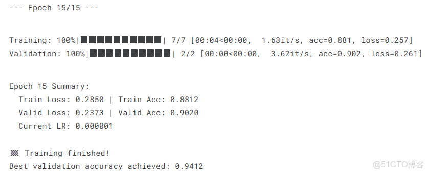
4.5模型評估
model = create_model()
model.load_state_dict(torch.load('best_model.pth', map_location=device))
model.to(device)
fig, (ax1, ax2) = plt.subplots(1, 2, figsize=(18, 6))
# Plot Training & Validation Accuracy
ax1.plot(history['train_acc'], label='Train Accuracy', color='royalblue')
ax1.plot(history['val_acc'], label='Validation Accuracy', color='darkorange')
ax1.set_title('Model Accuracy', fontsize=16)
ax1.set_xlabel('Epoch', fontsize=12)
ax1.set_ylabel('Accuracy', fontsize=12)
ax1.legend()
ax1.grid(True)
# Plot Training & Validation Loss
ax2.plot(history['train_loss'], label='Train Loss', color='royalblue')
ax2.plot(history['val_loss'], label='Validation Loss', color='darkorange')
ax2.set_title('Model Loss', fontsize=16)
ax2.set_xlabel('Epoch', fontsize=12)
ax2.set_ylabel('Loss', fontsize=12)
ax2.legend()
ax2.grid(True)
plt.suptitle('Training and Validation Learning Curves', fontsize=20)
plt.show()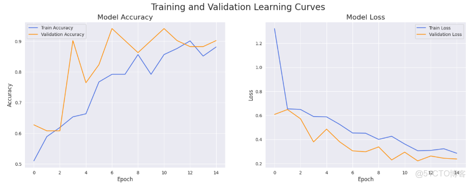
def get_predictions(model, data_loader, device):
model.eval()
all_preds = []
all_labels = []
all_probs = []
with torch.no_grad():
for images, labels in tqdm(data_loader, desc="Generating Predictions"):
images = images.to(device)
outputs = model(images).squeeze()
# Get probabilities for ROC curve
probs = torch.sigmoid(outputs)
# Get final predictions (0 or 1)
preds = (probs > 0.5).float()
all_preds.extend(preds.cpu().numpy())
all_labels.extend(labels.cpu().numpy())
all_probs.extend(probs.cpu().numpy())
return np.array(all_labels), np.array(all_preds), np.array(all_probs)
y_true, y_pred, y_prob = get_predictions(model, val_loader, device)target_names = ['No Tumor', 'Yes Tumor']
print("\n" + "="*50)
print(" Classification Report")
print("="*50 + "\n")
print(classification_report(y_true, y_pred, target_names=target_names))
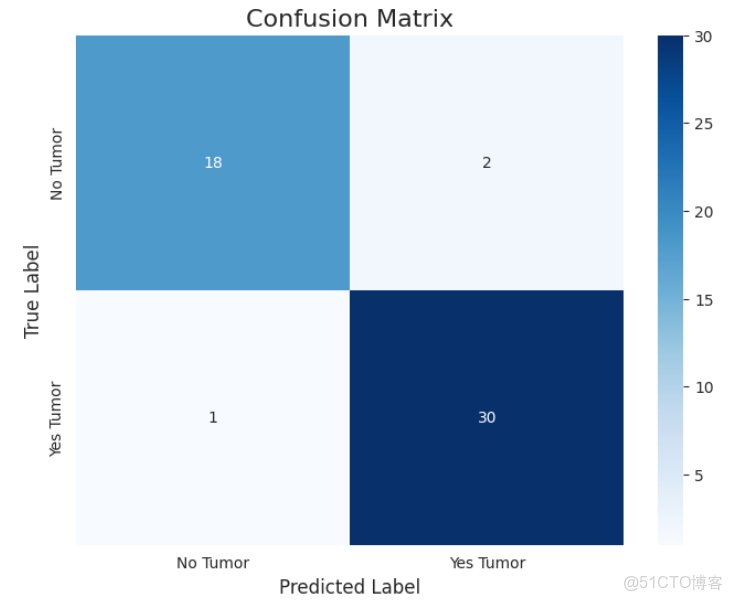
cm = confusion_matrix(y_true, y_pred)
plt.figure(figsize=(8, 6))
sns.heatmap(cm, annot=True, fmt='d', cmap='Blues',
xticklabels=target_names, yticklabels=target_names)
plt.title('Confusion Matrix', fontsize=16)
plt.xlabel('Predicted Label', fontsize=12)
plt.ylabel('True Label', fontsize=12)
plt.show()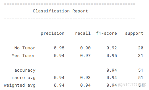
fpr, tpr, thresholds = roc_curve(y_true, y_prob)
roc_auc = auc(fpr, tpr)
plt.figure(figsize=(10, 8))
plt.plot(fpr, tpr, color='darkorange', lw=2, label=f'ROC curve (AUC = {roc_auc:.2f})')
plt.plot([0, 1], [0, 1], color='navy', lw=2, linestyle='--', label='No-Skill Line')
plt.xlim([0.0, 1.0])
plt.ylim([0.0, 1.05])
plt.xlabel('False Positive Rate', fontsize=12)
plt.ylabel('True Positive Rate', fontsize=12)
plt.title('Receiver Operating Characteristic (ROC) Curve', fontsize=16)
plt.legend(loc="lower right")
plt.grid(True)
plt.show()
print(f"\nArea Under the Curve (AUC): {roc_auc:.4f}")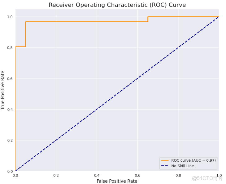
總體而言,在數據集中樣本數量有限的情況下,模型表現出了出色的性能,顯示了vit的強大!我們的AUC得分為0.971,CM和分類報告是令人滿意的。
4.6結果可視化
PATCH_SIZE = 16
def capture_attention_forward(self, x):
B, N, C = x.shape
qkv = self.qkv(x).reshape(B, N, 3, self.num_heads, C // self.num_heads).permute(2, 0, 3, 1, 4)
q, k, v = qkv.unbind(0)
attn = (q @ k.transpose(-2, -1)) * self.scale
attn = attn.softmax(dim=-1)
self.attention_map = attn
attn = self.attn_drop(attn)
x = (attn @ v).transpose(1, 2).reshape(B, N, C)
x = self.proj(x)
x = self.proj_drop(x)
return x
last_block = model.blocks[-1]
last_block.attn.forward = types.MethodType(capture_attention_forward, last_block.attn)
def visualize_attention(model, image_tensor, original_image, device, true_label, pred_label):
model.eval()
image_tensor = image_tensor.unsqueeze(0).to(device)
with torch.no_grad():
output = model(image_tensor)
attn_map = last_block.attn.attention_map
attn_map = attn_map.mean(dim=1).squeeze(0)
cls_token_attn = attn_map[0, 1:]
grid_size = int(np.sqrt(cls_token_attn.shape[0]))
attn_grid = cls_token_attn.cpu().numpy().reshape(grid_size, grid_size)
resized_attn = cv2.resize(attn_grid, (original_image.shape[1], original_image.shape[0]))
resized_attn = (resized_attn - resized_attn.min()) / (resized_attn.max() - resized_attn.min())
heatmap = cv2.applyColorMap(np.uint8(255 * resized_attn), cv2.COLORMAP_JET)
heatmap = cv2.cvtColor(heatmap, cv2.COLOR_BGR2RGB)
superimposed_img = cv2.addWeighted(original_image, 0.6, heatmap, 0.4, 0)
fig, (ax1, ax2, ax3) = plt.subplots(1, 3, figsize=(18, 6))
class_names = {0: 'No Tumor', 1: 'Yes Tumor'}
ax1.imshow(original_image)
ax1.set_title("Original Image", fontsize=14)
ax1.axis('off')
ax2.imshow(heatmap)
ax2.set_title("Attention Heatmap", fontsize=14)
ax2.axis('off')
ax3.imshow(superimposed_img)
ax3.set_title("Superimposed View", fontsize=14)
ax3.axis('off')
plt.suptitle(f"True: {class_names[true_label]} | Predicted: {class_names[pred_label]}", fontsize=18)
plt.show()
correct_yes_idx = np.where((y_true == 1) & (y_pred == 1))[0]
correct_no_idx = np.where((y_true == 0) & (y_pred == 0))[0]
incorrect_idx = np.where(y_true != y_pred)[0]
indices_to_show = []
if len(correct_yes_idx) > 0: indices_to_show.append(correct_yes_idx[0])
if len(correct_no_idx) > 0: indices_to_show.append(correct_no_idx[0])
if len(incorrect_idx) > 0: indices_to_show.append(incorrect_idx[0])
for idx in indices_to_show:
img_tensor, label = val_dataset[idx]
filepath = val_df.loc[idx, 'filepath']
original_img = np.array(Image.open(filepath).convert('RGB')) # Read with PIL
true_label = int(y_true[idx])
pred_label = int(y_pred[idx])
visualize_attention(model, img_tensor, original_img, device, true_label, pred_label)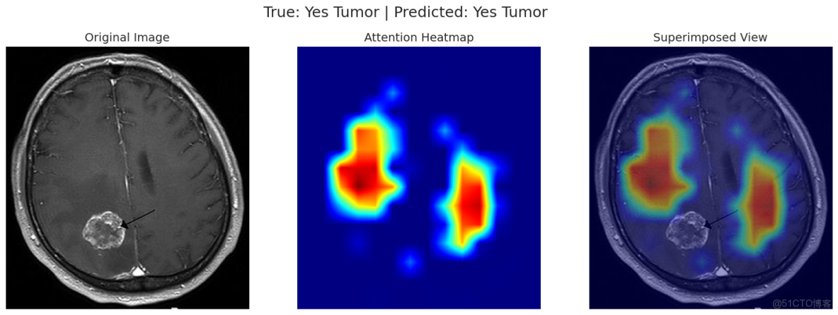
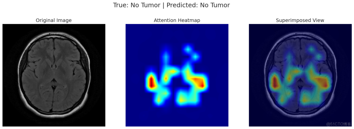
可以看出演示的這兩條數據模型均預測正確!
源代碼
import os
import cv2
import warnings
import timm
import torch
import copy
import types
import torch.nn as nn
import torch.optim as optim
import pandas as pd
import numpy as np
import albumentations as A
import matplotlib.pyplot as plt
import seaborn as sns
import plotly.express as px
from tqdm import tqdm
from PIL import Image
from collections import defaultdict
from sklearn.model_selection import StratifiedShuffleSplit
from sklearn.metrics import confusion_matrix, classification_report, roc_curve, auc
from albumentations.pytorch import ToTensorV2
from torch.utils.data import Dataset, DataLoader
from torch.optim.lr_scheduler import CosineAnnealingLR
sns.set_style("darkgrid")
warnings.filterwarnings('ignore')
DATA_DIR = './brain_tumor_dataset'
classes = [folder for folder in os.listdir(DATA_DIR) if os.path.isdir(os.path.join(DATA_DIR, folder))]
data = []
for cls in classes:
class_path = os.path.join(DATA_DIR, cls)
for filename in os.listdir(class_path):
filepath = os.path.join(class_path, filename)
data.append({'filepath': filepath, 'label': cls})
df = pd.DataFrame(data)
df = df.sample(frac=1).reset_index(drop=True)
print("First 5 rows of the DataFrame:")
display(df.head())
print("\n\nDataFrame Information:")
df.info()
print("\nClass Distribution:")
class_counts = df['label'].value_counts()
fig_pie = px.pie(
names=class_counts.index,
values=class_counts.values,
title='Class Distribution of Brain Tumor MRI',
color_discrete_sequence=px.colors.qualitative.Pastel
)
fig_pie.update_traces(textposition='inside', textinfo='percent+label')
fig_pie.show()
plt.figure(figsize=(8, 6))
sns.countplot(x='label', data=df, palette='viridis')
plt.title('Count of Images per Class')
plt.xlabel('Class Label')
plt.ylabel('Number of Images')
plt.show()
print(class_counts)
plt.figure(figsize=(15, 8))
n_samples = 5
yes_samples = df[df['label'] == 'yes'].sample(n_samples)

for i, row in enumerate(yes_samples.iterrows()):
    filepath = row[1]['filepath']
    img = cv2.imread(filepath)
    img = cv2.cvtColor(img, cv2.COLOR_BGR2RGB)
    plt.subplot(2, n_samples, i + 1)
    plt.imshow(img)
    plt.title(f"Tumor Detected\n(Class: yes)")
    plt.axis('off')


no_samples = df[df['label'] == 'no'].sample(n_samples)
for i, row in enumerate(no_samples.iterrows()):
    filepath = row[1]['filepath']
    img = cv2.imread(filepath)
    img = cv2.cvtColor(img, cv2.COLOR_BGR2RGB)
    plt.subplot(2, n_samples, n_samples + i + 1)
    plt.imshow(img)
    plt.title(f"No Tumor\n(Class: no)")
    plt.axis('off')

plt.tight_layout()
plt.show()
heights = []
widths = []
for filepath in tqdm(df['filepath'], desc="Reading image dimensions"):
try:
img = cv2.imread(filepath)
h, w, _ = img.shape
heights.append(h)
widths.append(w)
except Exception as e:
print(f"Could not read {filepath}: {e}")
df['height'] = heights
df['width'] = widths
print("\nStatistics for image dimensions:")
display(df[['height', 'width']].describe())
plt.figure(figsize=(14, 6))
plt.subplot(1, 2, 1)
sns.histplot(df['height'], kde=True, color='skyblue').set_title('Distribution of Image Heights')
plt.subplot(1, 2, 2)
sns.histplot(df['width'], kde=True, color='salmon').set_title('Distribution of Image Widths')
plt.show()
IMG_SIZE = 224
avg_yes = np.zeros((IMG_SIZE, IMG_SIZE, 3), np.float64)
avg_no = np.zeros((IMG_SIZE, IMG_SIZE, 3), np.float64)

count_yes = len(df[df['label'] == 'yes'])
count_no = len(df[df['label'] == 'no'])

for filepath in tqdm(df[df['label'] == 'yes']['filepath'], desc="Averaging 'yes' images"):
    img = cv2.imread(filepath)
    img = cv2.cvtColor(img, cv2.COLOR_BGR2RGB)
    img = cv2.resize(img, (IMG_SIZE, IMG_SIZE))
    avg_yes += img / count_yes

for filepath in tqdm(df[df['label'] == 'no']['filepath'], desc="Averaging 'no' images"):
    img = cv2.imread(filepath)
    img = cv2.cvtColor(img, cv2.COLOR_BGR2RGB)
    img = cv2.resize(img, (IMG_SIZE, IMG_SIZE))
    avg_no += img / count_no

avg_yes_img = np.array(np.round(avg_yes), dtype=np.uint8)
avg_no_img = np.array(np.round(avg_no), dtype=np.uint8)

print("\nDisplaying the 'average' brain MRI for each class:")
plt.figure(figsize=(12, 6))
plt.subplot(1, 2, 1)
plt.imshow(avg_no_img)
plt.title('Average Non-Tumorous Brain')
plt.axis('off')

plt.subplot(1, 2, 2)
plt.imshow(avg_yes_img)
plt.title('Average Tumorous Brain')
plt.axis('off')

plt.suptitle('Mean Image Representation by Class', fontsize=16)
plt.show()
IMG_SIZE = 224
BATCH_SIZE = 32
MEAN = [0.485, 0.456, 0.406]
STD = [0.229, 0.224, 0.225]

splitter = StratifiedShuffleSplit(n_splits=1, test_size=0.2, random_state=666)

for train_index, val_index in splitter.split(df, df['label']):
    train_df = df.iloc[train_index]
    val_df = df.iloc[val_index]

train_df = train_df.reset_index(drop=True)
val_df = val_df.reset_index(drop=True)

print("Training data info:")
print(train_df['label'].value_counts(normalize=True))
print("\nValidation data info:")
print(val_df['label'].value_counts(normalize=True))
train_transforms = A.Compose([
    A.Resize(IMG_SIZE, IMG_SIZE),
    A.HorizontalFlip(p=0.5),
    A.Rotate(limit=20, p=0.7),
    A.RandomBrightnessContrast(brightness_limit=0.2, contrast_limit=0.2, p=0.7),
    A.ElasticTransform(alpha=1, sigma=50, alpha_affine=50, p=0.5),
    A.CoarseDropout(max_holes=8, max_height=IMG_SIZE//8, max_width=IMG_SIZE//8,
                    min_holes=1, fill_value=0, p=0.5),
    A.Normalize(mean=MEAN, std=STD),
    ToTensorV2()
])

val_transforms = A.Compose([
    A.Resize(IMG_SIZE, IMG_SIZE),
    A.Normalize(mean=MEAN, std=STD),
    ToTensorV2()
])
class BrainMRIDataset(Dataset):
    def __init__(self, df, transforms=None):
        self.df = df
        self.transforms = transforms
        self.labels = self.df['label'].map({'yes': 1, 'no': 0}).values

    def __len__(self):
        return len(self.df)

    def __getitem__(self, idx):
        filepath = self.df.loc[idx, 'filepath']
        label = self.labels[idx]
        image = cv2.imread(filepath)
        image = cv2.cvtColor(image, cv2.COLOR_BGR2RGB)

        if self.transforms:
            transformed = self.transforms(image=image)
            image = transformed['image']

        return image, torch.tensor(label, dtype=torch.float32)
temp_train_dataset = BrainMRIDataset(train_df, transforms=train_transforms)
print("Visualizing some of the applied augmentations on a single training image:")

n_images = 8
original_image, _ = temp_train_dataset[0]
viz_transforms = A.Compose([t for t in temp_train_dataset.transforms if not isinstance(t, (A.Normalize, ToTensorV2))])

raw_img = cv2.imread(temp_train_dataset.df.loc[0, 'filepath'])
raw_img = cv2.cvtColor(raw_img, cv2.COLOR_BGR2RGB)

plt.figure(figsize=(16, 8))
plt.subplot(2, (n_images + 1) // 2, 1)
plt.imshow(raw_img)
plt.title("Original Image")
plt.axis('off')

for i in range(1, n_images):
    augmented = viz_transforms(image=raw_img)['image']
    plt.subplot(2, (n_images + 1) // 2, i + 1)
    plt.imshow(augmented)
    plt.title(f"Augmented {i}")
    plt.axis('off')

plt.tight_layout()
plt.show()
train_dataset = BrainMRIDataset(train_df, transforms=train_transforms)
val_dataset = BrainMRIDataset(val_df, transforms=val_transforms)

train_loader = DataLoader(train_dataset, batch_size=BATCH_SIZE, shuffle=True, num_workers=2)
val_loader = DataLoader(val_dataset, batch_size=BATCH_SIZE, shuffle=False, num_workers=2)

print(f"\nNumber of training batches: {len(train_loader)}")
print(f"Number of validation batches: {len(val_loader)}")

images, labels = next(iter(train_loader))
print(f"\nShape of one batch of images: {images.shape}")
print(f"Shape of one batch of labels: {labels.shape}")
MODEL_NAME = 'vit_base_patch16_224'
PRETRAINED = True
device = "cuda"

def create_model(num_classes=1):
    model = timm.create_model(MODEL_NAME, pretrained=PRETRAINED, num_classes=num_classes)
    in_features = model.head.in_features
    model.head = nn.Linear(in_features, num_classes)

    return model


model = create_model()
model.to(device)
print(f"\nModel '{MODEL_NAME}' loaded and adapted for binary classification.")
try:
    images, labels = next(iter(train_loader))
except NameError:
    print("DataLoaders not found. Creating dummy data for the smoke test.")
    images = torch.randn(BATCH_SIZE, 3, IMG_SIZE, IMG_SIZE)

images = images.to(device)
with torch.no_grad():
    output = model(images)

assert output.shape == (BATCH_SIZE, 1), f"Output shape is incorrect! Expected {(BATCH_SIZE, 1)}, but got {output.shape}"
EPOCHS = 15
LR = 1e-4
WEIGHT_DECAY = 1e-6

loss_fn = nn.BCEWithLogitsLoss()
optimizer = optim.AdamW(model.parameters(), lr=LR, weight_decay=WEIGHT_DECAY)
scheduler = CosineAnnealingLR(optimizer, T_max=len(train_loader) * EPOCHS, eta_min=1e-6)

def train_one_epoch(model, train_loader, loss_fn, optimizer, scheduler, device):
    model.train()
    running_loss = 0.0
    correct_predictions = 0
    total_samples = 0

    progress_bar = tqdm(train_loader, desc="Training", total=len(train_loader))

    for images, labels in progress_bar:
        images = images.to(device)
        labels = labels.to(device)

        outputs = model(images)
        outputs = outputs.squeeze()

        loss = loss_fn(outputs, labels)

        optimizer.zero_grad()
        loss.backward()
        optimizer.step()
        scheduler.step()

        running_loss += loss.item() * images.size(0)

        preds = (torch.sigmoid(outputs) > 0.5).float()
        correct_predictions += (preds == labels).sum().item()
        total_samples += labels.size(0)

        progress_bar.set_postfix(loss=loss.item(), acc=correct_predictions/total_samples)

    epoch_loss = running_loss / total_samples
    epoch_acc = correct_predictions / total_samples
    return epoch_loss, epoch_acc


def validate_one_epoch(model, val_loader, loss_fn, device):
    model.eval()
    running_loss = 0.0
    correct_predictions = 0
    total_samples = 0

    progress_bar = tqdm(val_loader, desc="Validation", total=len(val_loader))

    with torch.no_grad():
        for images, labels in progress_bar:
            images = images.to(device)
            labels = labels.to(device)

            outputs = model(images).squeeze()
            loss = loss_fn(outputs, labels)

            running_loss += loss.item() * images.size(0)

            preds = (torch.sigmoid(outputs) > 0.5).float()
            correct_predictions += (preds == labels).sum().item()
            total_samples += labels.size(0)

            progress_bar.set_postfix(loss=loss.item(), acc=correct_predictions/total_samples)

    epoch_loss = running_loss / total_samples
    epoch_acc = correct_predictions / total_samples
    return epoch_loss, epoch_acc
history = defaultdict(list)
best_val_acc = 0.0
best_model_state = None

print("🚀 Starting training!")
for epoch in range(1, EPOCHS + 1):
    print(f"\n--- Epoch {epoch}/{EPOCHS} ---")

    train_loss, train_acc = train_one_epoch(model, train_loader, loss_fn, optimizer, scheduler, device)
    val_loss, val_acc = validate_one_epoch(model, val_loader, loss_fn, device)

    print(f"Epoch {epoch} Summary:")
    print(f"  Train Loss: {train_loss:.4f} | Train Acc: {train_acc:.4f}")
    print(f"  Valid Loss: {val_loss:.4f} | Valid Acc: {val_acc:.4f}")
    print(f"  Current LR: {optimizer.param_groups[0]['lr']:.6f}")

    history['train_loss'].append(train_loss)
    history['train_acc'].append(train_acc)
    history['val_loss'].append(val_loss)
    history['val_acc'].append(val_acc)

    if val_acc > best_val_acc:
        best_val_acc = val_acc
        best_model_state = copy.deepcopy(model.state_dict())
        torch.save(best_model_state, 'best_model.pth')
        print(f"🎉 New best model saved with validation accuracy: {best_val_acc:.4f}")

print("\n🏁 Training finished!")
print(f"Best validation accuracy achieved: {best_val_acc:.4f}")
model = create_model()
model.load_state_dict(torch.load('best_model.pth', map_location=device))
model.to(device)
print("Best model loaded successfully for evaluation.")
fig, (ax1, ax2) = plt.subplots(1, 2, figsize=(18, 6))
# Plot Training & Validation Accuracy
ax1.plot(history['train_acc'], label='Train Accuracy', color='royalblue')
ax1.plot(history['val_acc'], label='Validation Accuracy', color='darkorange')
ax1.set_title('Model Accuracy', fontsize=16)
ax1.set_xlabel('Epoch', fontsize=12)
ax1.set_ylabel('Accuracy', fontsize=12)
ax1.legend()
ax1.grid(True)
# Plot Training & Validation Loss
ax2.plot(history['train_loss'], label='Train Loss', color='royalblue')
ax2.plot(history['val_loss'], label='Validation Loss', color='darkorange')
ax2.set_title('Model Loss', fontsize=16)
ax2.set_xlabel('Epoch', fontsize=12)
ax2.set_ylabel('Loss', fontsize=12)
ax2.legend()
ax2.grid(True)
plt.suptitle('Training and Validation Learning Curves', fontsize=20)
plt.show()
def get_predictions(model, data_loader, device):
    model.eval()
    all_preds = []
    all_labels = []
    all_probs = []

    with torch.no_grad():
        for images, labels in tqdm(data_loader, desc="Generating Predictions"):
            images = images.to(device)

            outputs = model(images).squeeze()

            # Get probabilities for ROC curve
            probs = torch.sigmoid(outputs)

            # Get final predictions (0 or 1)
            preds = (probs > 0.5).float()

            all_preds.extend(preds.cpu().numpy())
            all_labels.extend(labels.cpu().numpy())
            all_probs.extend(probs.cpu().numpy())

    return np.array(all_labels), np.array(all_preds), np.array(all_probs)

y_true, y_pred, y_prob = get_predictions(model, val_loader, device)
target_names = ['No Tumor', 'Yes Tumor']
print("\n" + "="*50)
print("           Classification Report")
print("="*50 + "\n")
print(classification_report(y_true, y_pred, target_names=target_names))

cm = confusion_matrix(y_true, y_pred)

plt.figure(figsize=(8, 6))
sns.heatmap(cm, annot=True, fmt='d', cmap='Blues',
            xticklabels=target_names, yticklabels=target_names)
plt.title('Confusion Matrix', fontsize=16)
plt.xlabel('Predicted Label', fontsize=12)
plt.ylabel('True Label', fontsize=12)
plt.show()
fpr, tpr, thresholds = roc_curve(y_true, y_prob)
roc_auc = auc(fpr, tpr)

plt.figure(figsize=(10, 8))
plt.plot(fpr, tpr, color='darkorange', lw=2, label=f'ROC curve (AUC = {roc_auc:.2f})')
plt.plot([0, 1], [0, 1], color='navy', lw=2, linestyle='--', label='No-Skill Line')
plt.xlim([0.0, 1.0])
plt.ylim([0.0, 1.05])
plt.xlabel('False Positive Rate', fontsize=12)
plt.ylabel('True Positive Rate', fontsize=12)
plt.title('Receiver Operating Characteristic (ROC) Curve', fontsize=16)
plt.legend(loc="lower right")
plt.grid(True)
plt.show()

print(f"\nArea Under the Curve (AUC): {roc_auc:.4f}")
PATCH_SIZE = 16
def capture_attention_forward(self, x):
B, N, C = x.shape
qkv = self.qkv(x).reshape(B, N, 3, self.num_heads, C // self.num_heads).permute(2, 0, 3, 1, 4)
q, k, v = qkv.unbind(0)
attn = (q @ k.transpose(-2, -1)) * self.scale
attn = attn.softmax(dim=-1)
self.attention_map = attn
attn = self.attn_drop(attn)
x = (attn @ v).transpose(1, 2).reshape(B, N, C)
x = self.proj(x)
x = self.proj_drop(x)
return x
last_block = model.blocks[-1]
last_block.attn.forward = types.MethodType(capture_attention_forward, last_block.attn)
print("Model has been patched to capture attention maps.")
def visualize_attention(model, image_tensor, original_image, device, true_label, pred_label):
"""
Generates and displays the attention map for a given image.
"""
model.eval()
image_tensor = image_tensor.unsqueeze(0).to(device)
with torch.no_grad():
output = model(image_tensor)
attn_map = last_block.attn.attention_map
attn_map = attn_map.mean(dim=1).squeeze(0)
cls_token_attn = attn_map[0, 1:]
grid_size = int(np.sqrt(cls_token_attn.shape[0]))
attn_grid = cls_token_attn.cpu().numpy().reshape(grid_size, grid_size)
resized_attn = cv2.resize(attn_grid, (original_image.shape[1], original_image.shape[0]))
resized_attn = (resized_attn - resized_attn.min()) / (resized_attn.max() - resized_attn.min())
heatmap = cv2.applyColorMap(np.uint8(255 * resized_attn), cv2.COLORMAP_JET)
heatmap = cv2.cvtColor(heatmap, cv2.COLOR_BGR2RGB)
superimposed_img = cv2.addWeighted(original_image, 0.6, heatmap, 0.4, 0)
fig, (ax1, ax2, ax3) = plt.subplots(1, 3, figsize=(18, 6))
class_names = {0: 'No Tumor', 1: 'Yes Tumor'}
ax1.imshow(original_image)
ax1.set_title("Original Image", fontsize=14)
ax1.axis('off')
ax2.imshow(heatmap)
ax2.set_title("Attention Heatmap", fontsize=14)
ax2.axis('off')
ax3.imshow(superimposed_img)
ax3.set_title("Superimposed View", fontsize=14)
ax3.axis('off')
plt.suptitle(f"True: {class_names[true_label]} | Predicted: {class_names[pred_label]}", fontsize=18)
plt.show()
correct_yes_idx = np.where((y_true == 1) & (y_pred == 1))[0]
correct_no_idx = np.where((y_true == 0) & (y_pred == 0))[0]
incorrect_idx = np.where(y_true != y_pred)[0]
indices_to_show = []
if len(correct_yes_idx) > 0: indices_to_show.append(correct_yes_idx[0])
if len(correct_no_idx) > 0: indices_to_show.append(correct_no_idx[0])
if len(incorrect_idx) > 0: indices_to_show.append(incorrect_idx[0])
for idx in indices_to_show:
img_tensor, label = val_dataset[idx]
filepath = val_df.loc[idx, 'filepath']
original_img = np.array(Image.open(filepath).convert('RGB')) # Read with PIL
true_label = int(y_true[idx])
pred_label = int(y_pred[idx])
visualize_attention(model, img_tensor, original_img, device, true_label, pred_label)