什麼是激活函數
激活函數,屬於神經網絡中的概念。
激活函數,就像神經元的開關,決定了輸入信號能否被傳遞,以及以什麼形式傳遞。
為應對不同的場景,激活函數不斷髮展出了各種實現。它們存在的意義,就是為信號傳遞賦予不同種類的“非線性”特徵,從而讓神經網絡能夠表達更為豐富的含義。
本文旨在梳理常見的 40 多種激活函數(也包含少量經典的輸出層函數)。
説明
本文將簡要介紹激活函數的概念和使用場景,並列出其數學公式,然後基於Python進行可視化實現。最後一節則以表格的形式,從多個維度對比了其中最為經典的 20 多個激活函數,以期為讀者提供選型參考。
本文所有代碼實現均基於Jupyter NoteBook,感興趣的讀者可以後台留言獲取完整ipynb文件。
為使得各激活函數的代碼實現更為簡潔,首先做一些初始化操作,如導入對應Python庫、定義對應的繪圖函數等,如下:
# -*- coding: utf-8 -*-

# 導入必要的庫
import numpy as np
import matplotlib.pyplot as plt
from scipy.special import expit as sigmoid  # scipy 的 sigmoid
import warnings
warnings.filterwarnings("ignore")

# 設置中文字體和圖形樣式
plt.rcParams['font.sans-serif'] = ['SimHei', 'Arial Unicode MS', 'DejaVu Sans']
plt.rcParams['axes.unicode_minus'] = False
plt.style.use('seaborn-v0_8')  # 使用美觀樣式
# 定義輸入範圍
x = np.linspace(-10, 10, 1000)

# 定義畫圖函數(單張圖)
def plot_activation(func, grad_func, name):
    y = func(x)
    dy = grad_func(x)
    plt.figure(figsize=(8, 5))
    plt.plot(x, y, label=name, linewidth=1.5)
    plt.plot(x, dy, label=f"{name}'s derivative", linestyle='--', linewidth=1.5)
    plt.title(f'{name} Function and Its Derivative')
    plt.legend()
    plt.grid(True)
    plt.axhline(0, color='black', linewidth=0.5)
    plt.axvline(0, color='black', linewidth=0.5)
    plt.show()


# 定義畫圖函數(多張圖,用於對比不同參數的效果)
def plot_activations(functions, x):
    plt.figure(figsize=(10, 7))
    for func, grad_func, name in functions:
        y = func(x)
        dy = grad_func(x)
        plt.plot(x, y, label=name, linewidth=1.5)
        plt.plot(x, dy, label=f"{name}'s derivative", linestyle='--', linewidth=1.5)

    plt.title('Activation Functions and Their Derivatives')
    plt.legend()
    plt.grid(True)
    plt.axhline(0, color='black', linewidth=0.5)
    plt.axvline(0, color='black', linewidth=0.5)
    plt.show()
接下來,讓我們開始吧!
經典激活函數
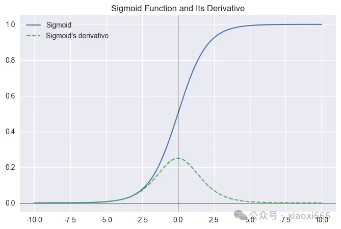
Sigmoid
適用於二分類問題的輸出層,將輸出壓縮到 (0,1) 區間表示概率。不推薦用於隱藏層,因易導致梯度消失。
公式
實現
def sigmoid(x):
    return 1 / (1 + np.exp(-x))

def sigmoid_grad(x):
    s = sigmoid(x)
    return s * (1 - s)

plot_activation(sigmoid, sigmoid_grad, 'Sigmoid')
圖像
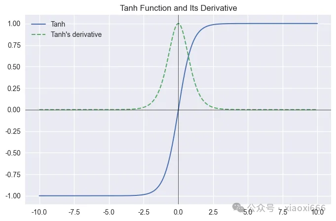
Tanh(雙曲正切)
Tanh 輸出零中心化,使梯度更新方向更均衡,收斂更快,是一種比 Sigmoid 更優的激活函數,適合隱藏層使用,尤其在 RNN 中仍有應用。但它仍可能梯度消失。
公式
實現
def tanh(x):
    return np.tanh(x)

def tanh_grad(x):
    return 1 - np.tanh(x)**2

plot_activation(tanh, tanh_grad, 'Tanh')
圖像
Linear
主要用於迴歸任務的輸出層,保持輸出為原始實數,不進行非線性變換。
不適合用在隱藏層(否則整個網絡等價於單層線性模型,無法學習非線性特徵)。
在某些特定模型(如自編碼器的中間層或策略網絡)中也可能使用。
公式
實現
def linear(x):
    return x

def linear_grad(x):
    return np.ones_like(x)

plot_activation(linear, linear_grad, 'Linear')
圖像

Softmax
多分類問題的輸出層標準激活函數,將輸出轉化為概率分佈。不用於隱藏層。
公式
實現
from mpl_toolkits.mplot3d import Axes3D

def softmax(x):
    exp_x = np.exp(x - np.max(x, axis=0, keepdims=True))  # 數值穩定
    return exp_x / np.sum(exp_x, axis=0, keepdims=True)

def softmax_grad(x):
    s = softmax(x).reshape(-1, 1)
    return np.diagflat(s) - np.dot(s, s.T)  # Jacobian矩陣

# 生成輸入數據(二維,便於可視化)
x = np.linspace(-10, 10, 100)
y = np.linspace(-10, 10, 100)
X, Y = np.meshgrid(x, y)
inputs = np.vstack([X.ravel(), Y.ravel()]).T

# 計算Softmax輸出(取第一個維度作為輸出值,因為Softmax輸出是概率分佈)
outputs = np.array([softmax(p)[0] for p in inputs]).reshape(X.shape)

# 計算梯度(取Jacobian矩陣的第一個對角線元素)
gradients = np.array([softmax_grad(p)[0, 0] for p in inputs]).reshape(X.shape)

# 繪製Softmax函數
fig = plt.figure(figsize=(12, 5))

# 1. Softmax函數圖像
ax1 = fig.add_subplot(121, projection='3d')
ax1.plot_surface(X, Y, outputs, cmap='viridis', alpha=0.8)
ax1.set_title('Softmax (First Output Dimension)')
ax1.set_xlabel('x1')
ax1.set_ylabel('x2')
ax1.set_zlabel('P(x1)')

# 2. Softmax梯度圖像
ax2 = fig.add_subplot(122, projection='3d')
ax2.plot_surface(X, Y, gradients, cmap='plasma', alpha=0.8)
ax2.set_title('Gradient of Softmax (∂P(x1)/∂x1)')
ax2.set_xlabel('x1')
ax2.set_ylabel('x2')
ax2.set_zlabel('Gradient')

plt.tight_layout()
plt.show()
圖像

ReLU 函數及其變體
ReLU(Rectified Linear Unit)
中文名稱是線性整流函數,是在神經網絡中常用的激活函數。通常意義下,其指代數學中的斜坡函數。
公式
實現
def relu(x):
    return np.maximum(0, x)

def relu_grad(x):
    return (x > 0).astype(float)

plot_activation(relu, relu_grad, 'RelU')
圖像

ReLU6
ReLU6 是 ReLU 的有界版本,輸出限制在 [0, 6] 區間。
主要用於移動端和輕量級網絡(如 MobileNet、EfficientNet 的早期版本),其有界性有助於提升低精度推理(如量化)時的穩定性。
也常見於強化學習(如 DQN)中,用於限制輸出範圍,防止訓練波動。
公式
或:
實現
def relu6(x):
    return np.minimum(np.maximum(0, x), 6)

def relu6_grad(x):
    dx = np.zeros_like(x)
    dx[(x > 0) & (x < 6)] = 1
    return dx

plot_activation(relu6, relu6_grad, 'ReLU6')
圖像

Leaky ReLU
Leaky ReLU 是對傳統 ReLU 的改進,它試圖解決“死亡 ReLU”問題,即某些神經元可能永遠不會再激活的問題。
公式
通常固定取實現
def leaky_relu(x, alpha=0.01):
    return np.where(x > 0, x, x * alpha)

def leaky_relu_grad(x, alpha=0.1):
    dx = np.ones_like(x)
    dx[x < 0] = alpha
    return dx

plot_activation(leaky_relu, leaky_relu_grad, 'Leaky ReLU')
圖像

PReLU(Parametric ReLU)
上一節的 Leaky ReLU 是“固定小斜率”,而 PReLU 將該斜率變為可學習參數,表達能力更強。
公式
實現
def prelu(x, alpha=0.25):
    return np.where(x > 0, x, alpha * x)

def prelu_grad(x, alpha=0.25):
    return np.where(x > 0, 1, alpha)

functions_to_plot = [
    (lambda x: prelu(x, 0.1), lambda x: prelu_grad(x, 0.1), 'PReLU α=0.1'),
    (lambda x: prelu(x, 0.25), lambda x: prelu_grad(x, 0.25), 'PReLU α=0.25'),
    (lambda x: prelu(x, 0.5), lambda x: prelu_grad(x, 0.5), 'PReLU α=0.5')
]
plot_activations(functions_to_plot, x)
圖像

RReLU(Randomized ReLU)
RReLU是一種在訓練時使用隨機斜率的變體ReLU激活函數,而在測試時則採用固定的斜率。其主要目的是為了減少過擬合併解決“死亡ReLU”問題。
由於 RReLU 在訓練時使用的是一個區間內的隨機值,而測試時使用的是固定值。為了簡化起見,這裏使用一個確定性的斜率(例如訓練過程中使用的平均斜率)。
以下代碼實現了 RReLU 函數及其導數,並使用了一個介於 lower 和 upper 之間的固定斜率來代替隨機選擇的過程,以便進行可視化。
在實際應用中,對於每個負輸入值,斜率會在給定範圍內隨機選擇,但在測試或推理階段,通常會使用所有可能斜率的平均值。
實現
def rrelu(x, lower=1/8., upper=1/3.):
    # 在實際應用中,這裏的a應該是在[lower, upper]之間隨機選取的
    # 但為了繪圖方便,我們取平均值作為固定的a
    a = (lower + upper) / 2
    return np.where(x >= 0, x, a * x)

def rrelu_grad(x, lower=1/8., upper=1/3.):
    a = (lower + upper) / 2
    dx = np.ones_like(x)
    dx[x < 0] = a
    return dx

plot_activation(lambda x: rrelu(x), lambda x: rrelu_grad(x), 'RReLU')
圖像

ELU(Exponential Linear Unit)
ELU 旨在解決傳統激活函數在深度神經網絡中可能遇到的一些問題,例如梯度消失和“死亡神經元”問題。
它能產生負值輸出,使激活均值接近零,加速收斂。適合深層網絡,訓練穩定性優於 ReLU,但計算稍慢。
公式
實現
def elu(x, alpha=1.0):
    return np.where(x > 0, x, alpha * (np.exp(x) - 1))

def elu_grad(x, alpha=1.0):
    return np.where(x > 0, 1, elu(x, alpha) + alpha)

functions_to_plot = [
    (lambda x: elu(x, 0.1), lambda x: elu_grad(x, 0.1), 'ELU α=0.1'),
    (lambda x: elu(x, 0.25), lambda x: elu_grad(x, 0.25), 'ELU α=0.25'),
    (lambda x: elu(x, 0.5), lambda x: elu_grad(x, 0.5), 'ELU α=0.5'),
    (lambda x: elu(x, 1), lambda x: elu_grad(x,1), 'ELU α=1'),
    (lambda x: elu(x, 2), lambda x: elu_grad(x,2), 'ELU α=2')
]
plot_activations(functions_to_plot, x)
圖像

SELU(Scaled Exponential Linear Units)
SELU 是一種自歸一化激活函數,它能夠使得神經網絡的輸出在一定條件下自動趨近於零均值和單位方差,從而有助於加速訓練過程,並且有可能提高模型的性能。
SELU激活函數是由Günter Klambauer等人在2017年的論文《Self-Normalizing Neural Networks》中提出的。
公式
實現
# SELU 參數(論文中推薦值)
lambda_s = 1.0507009873554804934193349852946
alpha_s = 1.673261549988240216825385979984

def selu(x, lambda_=1.0507009873554804934193349852946, alpha=1.673261549988240216825385979984):
    return lambda_ * np.where(x > 0, x, alpha * (np.exp(x) - 1))

def selu_grad(x, lambda_=1.0507009873554804934193349852946, alpha=1.673261549988240216825385979984):
    return lambda_ * np.where(x > 0, 1, alpha * np.exp(x))

# 調用plot_activation繪製SELU及其導數
plot_activation(lambda x: selu(x), lambda x: selu_grad(x), 'SELU')
圖像

CELU(Continuously Differentiable Exponential Linear Unit)
CELU 是 ELU 的改進版本,保證了在 x = 0 處連續可導(平滑性優於 ELU),有助於優化穩定性。
與 ELU 類似,能產生負值激活,促進神經元平均輸出接近零,適合深層網絡訓練。在某些對梯度平滑性要求較高的任務中可作為 ReLU、ELU 的替代選擇,但計算成本略高。
公式
實現
def celu(x, alpha=1.0):
    return np.where(x > 0, x, alpha * (np.exp(x / alpha) - 1))

def celu_grad(x, alpha=1.0):
    dx = np.ones_like(x)
    dx[x <= 0] = np.exp(x[x <= 0] / alpha)
    return dx

plot_activation(celu, celu_grad, "CELU")
圖像

GELU (Gaussian Error Linear Unit,高斯誤差線性單元)
GELU 是 Transformer 等現代架構(如 BERT)的標準激活函數,平滑且非單調,在 NLP 和大模型中廣泛使用。它的性能優於 ReLU,逐漸成為ReLU的替代選擇。
GELU 是由 Dan Hendrycks 和 Kevin Gimpel 在2016年的論文《Gaussian Error Linear Units (GELUs)》中提出。
公式
其中,
可以用雙曲正切函數(tanh)近似表示,常見形式為:
因此,實際計算中經常使用近似公式:
實現
def gelu(x):
    return 0.5 * x * (1 + np.tanh(np.sqrt(2 / np.pi) * (x + 0.044715 * np.power(x, 3))))

def gelu_grad(x):
    # 導數計算較為複雜,這裏簡化處理
    return 0.5 * (1 + np.tanh(np.sqrt(2 / np.pi) * (x + 0.044715 * np.power(x, 3)))) + \
           0.5 * x * (1 - np.tanh(np.sqrt(2 / np.pi) * (x + 0.044715 * np.power(x, 3)))**2) * \
           (np.sqrt(2 / np.pi) * (1 + 0.134145 * np.power(x, 2)))

plot_activation(gelu, gelu_grad, "GELU")
圖像

現代高性能激活函數
Swish
由 Google 提出,在某些深度模型中表現優於 ReLU,尤其在注意力機制和移動端模型中有效。
公式
其中,
而 β 是一個可學習參數。
實現
def swish(x, beta=1):
    return x / (1 + np.exp(-beta*x))

def swish_grad(x, beta=1):
    s = 1 / (1 + np.exp(-beta*x))
    f = x * s
    return f + (s * (1 - f)) * beta

plot_activation(swish, swish_grad, "Swish")
圖像

SiLU(Sigmoid Linear Unit)
SiLU 是 Swish 激活函數在 (beta=1) 時的特例。
實現與圖像可參考 Swish。
E-Swish
E-Swish 是 SiLU 的縮放版本,通過超參數 (beta) 增強非線性表達能力。
實現
假設 beta 為1.5:
def eswish(x, beta=1.5):
    return beta * x * sigmoid(x)

def eswish_grad(x, beta=1.5):
    s = sigmoid(x)
    return beta * s * (1 + x * (1 - s))

plot_activation(lambda x: eswish(x, beta=1.5), lambda x: eswish_grad(x, beta=1.5), 'E-Swish')
圖像

Mish
Mish 是一種自門控(self-gated)的非單調激活函數,由Diganta Misra在2019年的論文《Mish: A Self Regularized Non-Monotonic Neural Activation Function》中提出。
它在深度學習中表現出色,尤其在圖像分類等任務中,性能常優於ReLU及其變體(如Swish、Leaky ReLU等)。
公式
實現
def mish(x):
    return x * np.tanh(np.log(1 + np.exp(x)))

def mish_grad(x):
    sp = np.log(1 + np.exp(x))
    tanh_sp = np.tanh(sp)
    sech2_sp = 1 - tanh_sp**2
    return tanh_sp + x * sech2_sp * sigmoid(x)

plot_activation(mish, mish_grad, 'Mish')
圖像

SQNL(Square Nonlinearity)
SQNL 激活函數使用平方算子引入所需的非線性,其特點是計算操作次數更少。其在多層感知器人工神經網絡架構問題中的收斂速度更快。此外,該函數的導數是線性的,因此梯度計算速度更快。
SQNL 激活函數是由Adedamola Wuraola等人在2018年的論文《SQNL: A New Computationally Efficient Activation Function》中提出的。
公式
實現
def sqnl(x):
    return np.where(x > 2, 1,
           np.where(x >= 0, x - (x**2)/4,
           np.where(x >= -2, x + (x**2)/4, -1)))

def sqnl_grad(x):
    return np.where(x > 2, 0,
           np.where(x >= 0, 1 - x/2,
           np.where(x >= -2, 1 + x/2, 0)))

plot_activation(sqnl, sqnl_grad, 'SQNL')
圖像

Bent Identity
Bent Identity 是一種平滑、非單調、可微、無上界的激活函數,輸出接近輸入值但帶有輕微非線性彎曲(“bent”)。
它適用於迴歸任務或自編碼器的隱藏層,尤其在需要保留輸入結構的同時引入輕微非線性變換的場景。其導數始終大於 0.5,避免梯度消失,適合淺層網絡或需要穩定梯度的訓練過程。
但由於計算涉及平方根,速度較慢,不常用於大規模深度網絡。
另可參閲:https://www.gabormelli.com/RKB/Bent_Identity_Activation_Function
公式
實現
def bent_identity(x):
    return (np.sqrt(x**2 + 1) - 1) / 2 + x

def bent_identity_grad(x):
    return x / (2 * np.sqrt(x**2 + 1)) + 1

plot_activation(bent_identity, bent_identity_grad, 'Bent Identity')
圖像

門控與組合型激活函數
GLU (Gated Linear Unit)
GLU 是一種門控機制激活函數,通過將輸入的一部分作為“門”來調製另一部分的輸出,增強了模型的表達能力。
GLU 廣泛應用於 Transformer 變體(如 GLU Variants in GLU-Transformer)、序列模型(如 CNN-based NLP 模型)和語音任務中。
相比傳統激活函數,GLU 能更靈活地控制信息流動,提升建模能力。常見變體包括 SwiGLU、ReLU-Glu 等,在大模型(如 Llama 系列)中表現優異。
公式
實現
import numpy as np
import matplotlib.pyplot as plt
from mpl_toolkits.mplot3d import Axes3D


def glu_2d(x):
    """二維輸入版本的GLU"""
    a, b = x[..., 0], x[..., 1]  # 分割輸入的兩個維度
    return a * sigmoid(b)

def plot_glu_2d():
    # 創建二維輸入網格
    x = np.linspace(-4, 4, 50)
    y = np.linspace(-4, 4, 50)
    X, Y = np.meshgrid(x, y)
    xy = np.stack([X, Y], axis=-1)  # 組合成(50,50,2)的輸入

    # 計算GLU輸出
    Z = glu_2d(xy)

    # 3D可視化
    fig = plt.figure(figsize=(12, 6))

    # 1. 激活函數曲面
    ax1 = fig.add_subplot(121, projection='3d')
    ax1.plot_surface(X, Y, Z, cmap='viridis', alpha=0.8)
    ax1.set_title('GLU: a * σ(b)')
    ax1.set_xlabel('Input a')
    ax1.set_ylabel('Input b')
    ax1.set_zlabel('Output')

    # 2. 梯度場切片(固定b=0時的梯度)
    ax2 = fig.add_subplot(122)
    b_zero_idx = np.abs(y).argmin()  # 找到b=0的索引
    grad_at_b0 = Z[b_zero_idx] * (1 - Z[b_zero_idx])  # ∂(aσ(b))/∂a = σ(b)
    ax2.plot(x, grad_at_b0, label='∂GLU/∂a at b=0', color='blue')
    ax2.plot(x, np.zeros_like(x), label='∂GLU/∂b at b=0', color='red')
    ax2.set_title('Gradient Slices at b=0')
    ax2.legend()
    ax2.grid(True)

    plt.tight_layout()
    plt.show()

# 執行可視化
plot_glu_2d()
圖像

Maxout
Maxout 是一種分段線性激活函數,定義為多個線性變換的最大值。它是一種可學習的分段線性激活函數,具有很強的表達能力——理論上,只要有足夠多的片段,它可以逼近任意凸函數。
它與 Dropout 結合使用時表現優異,曾廣泛用於全連接網絡。但由於每個 Maxout 單元需要 k 倍參數(即 k 個 W_i, b_i),參數量大、計算開銷高,因此在現代 CNN 或大模型中較少使用。適合對模型表達力要求高、但對計算資源不敏感的研究性任務。
公式
實現
def maxout(x, w1=1.0, w2=-1.0, b1=0.0, b2=0.0):
    """
    Maxout 簡化版(k=2)用於可視化:
    f(x) = max(w1*x + b1, w2*x + b2)

    常用設置:w1=1, w2=-1 → f(x) = max(x, -x) = |x|(絕對值)
    """
    return np.maximum(w1 * x + b1, w2 * x + b2)

def maxout_grad(x, w1=1.0, w2=-1.0, b1=0.0, b2=0.0):
    """
    Maxout 梯度:根據哪個線性函數被激活返回對應權重
    """
    linear1 = w1 * x + b1
    linear2 = w2 * x + b2
    return np.where(linear1 >= linear2, w1, w2)

# 可視化:f(x) = max(x, -x) = |x|
plot_activation(lambda x: maxout(x, w1=1.0, w2=-1.0),
                lambda x: maxout_grad(x, w1=1.0, w2=-1.0),
                'Maxout (k=2, |x|)')
圖像

SReLU (S-shaped Rectified Linear Unit)
SReLU 是一種參數自適應的 S 形激活函數,能夠根據數據自動學習激活曲線的形狀,兼具線性和飽和特性。適用於需要靈活非線性變換的全連接網絡或卷積網絡,在某些圖像分類和迴歸任務中表現優於 ReLU 和 ELU。
其設計目標是模擬生物神經元的響應特性,在深度模型中可提升表達能力。
但由於引入了四個可學習參數(每通道或共享),增加了模型複雜度,訓練成本較高,目前應用不如 ReLU 或 GELU 廣泛。
公式
實現
def srelu(x, tl=0.0, al=0.01, tr=1.0, ar=0.01):
    return np.where(x <= tl, tl + al * (x - tl),
           np.where(x < tr, x,
                    tr + ar * (x - tr)))

def srelu_grad(x, tl=0.0, al=0.01, tr=1.0, ar=0.01):
    return np.where(x <= tl, al,
           np.where(x < tr, 1.0, ar))

plot_activation(lambda x: srelu(x, tl=0.0, al=0.01, tr=1.0, ar=0.01),
                lambda x: srelu_grad(x, tl=0.0, al=0.01, tr=1.0, ar=0.01),
                'SReLU')
圖像

CReLU (Concatenated ReLU)
CReLU 是一種受“CNN模型中濾光片成對”啓發而發展出來的一種改進 ReLU 激活函數。由Wenling Shang等人於2016年在論文《Understanding and Improving Convolutional Neural Networks via Concatenated Rectified Linear Units》中提出。
公式
實現
def crelu(x):
    """
    輸出維度翻倍
    """
    return np.concatenate([relu(x), relu(-x)], axis=-1)

def crelu_grad(x):
    """
    CReLU 梯度:返回 [d/dx ReLU(x), d/dx ReLU(-x)]

    注意:ReLU(-x) 對 x 的導數是:
        - 如果 x < 0: ReLU(-x) = -x, 導數為 -1
        - 如果 x >= 0: ReLU(-x) = 0, 導數為 0
        => 即: -LeakyReLU(-x, negative_slope=1) 或 -H(x<0)

    所以:
        d/dx ReLU(-x) = -1 if x < 0 else 0
    """
    grad_positive = relu_grad(x)           # ReLU(x) 的梯度: 1 if x > 0 else 0
    grad_negative = np.where(x < 0, -1, 0) # ReLU(-x) 的梯度: -1 if x < 0 else 0

    return np.concatenate([grad_positive, grad_negative], axis=-1)

def plot_crelu_separate():
    x = np.linspace(-3, 3, 1000)
    y = crelu(x)
    grad = crelu_grad(x)

    plt.figure(figsize=(12, 5))

    plt.subplot(1, 2, 1)
    plt.plot(x, y[:len(x)], label='ReLU(x)')
    plt.plot(x, y[len(x):], label='ReLU(-x)')
    plt.title('CReLU: [ReLU(x), ReLU(-x)]')
    plt.legend()
    plt.grid(True)

    plt.subplot(1, 2, 2)
    plt.plot(x, grad[:len(x)], label="d/dx ReLU(x)", linestyle='--',)
    plt.plot(x, grad[len(x):], label="d/dx ReLU(-x)", linestyle='--',)
    plt.title('CReLU Gradient')
    plt.legend()
    plt.grid(True)

    plt.tight_layout()
    plt.show()

plot_crelu_separate()
圖像

特殊用途與研究型函數
Softplus
Softplus 是 ReLU 的平滑近似版本,輸出始終為正,且處處連續可導。當 x 很大時趨近於 x,當 x 很小時趨近於 0。
適用於需要平滑、非線性、非飽和(無上界)激活的場景,如:
- 變分自編碼器(VAE)中用於生成方差參數(保證正值);
- 強化學習中的策略網絡輸出層;
- 需要避免 ReLU “神經元死亡” 問題但又希望保持單側軟飽和特性的任務。
其主要缺點是計算開銷較大(涉及指數和對數),且在 x 很大時可能產生數值溢出,需做穩定處理(如 torch.nn.Softplus 內部實現會做裁剪)。
作為理論性質良好的激活函數,常用於概率建模和生成模型中。
公式
實現
def softplus(x):
    return np.log(1 + np.exp(x))

def softplus_grad(x):
    return sigmoid(x)

plot_activation(softplus, softplus_grad, 'Softplus')
圖像

Softsign
Softsign 是 Tanh 的替代品,輸出範圍 (−1,1),具有平滑的S形曲線但計算更簡單。
應用場景主要有:
- 替代Tanh/Sigmoid:需平滑飽和激活時(如RNN、生成模型)。
- 對抗梯度消失:梯度衰減比Tanh更緩慢,適合深層網絡。
- 低精度訓練:計算無指數運算,對量化友好。
優點:
- 計算高效:僅需一次除法和絕對值運算(比Tanh快約2倍)。
- 梯度平緩:最大梯度為1(對比Tanh的0.25),緩解梯度消失。
- 輸出歸一化:天然將輸入壓縮到(−1,1),避免數值爆炸。
缺點:
- 飽和區梯度趨零:當∣x∣→∞ 時梯度接近0,可能拖慢訓練。
- 非零中心化:輸出均值不為零(類似Sigmoid),需配合BatchNorm。
- 表達能力有限:非線性弱於Swish等新型激活函數。
公式
實現
def softsign(x):
    return x / (1 + np.abs(x))

def softsign_grad(x):
    return 1 / ((1 + np.abs(x)) ** 2)

plot_activation(softsign, softsign_grad, "Softsign")
圖像

Sine
Sine 是一種週期性、有界、平滑振盪的激活函數。與 ReLU、Sigmoid 等傳統激活函數不同,它具有無限多的極值點和零點,能自然地建模週期性或高頻信號。
主要適用於:
- 神經隱式表示(Neural Implicit Representations),如 SIREN(Sinusoidal Representation Networks),用於表示圖像、音頻、3D 形狀等連續信號;
- 函數逼近任務,尤其是包含週期性、振盪行為的物理系統建模(如波函數、機械振動);
- 需要高頻率細節重建的場景(如超分辨率、神經輻射場 NeRF 的變體)。
雖然不適用於通用深度分類網絡,但在特定科學計算和表示學習任務中表現出色。
公式
實現
def sine(x):
    return np.sin(x)

def sine_grad(x):
    return np.cos(x)

plot_activation(sine, sine_grad, "Sine")
圖像

Cosine
Cosine 是一種週期性、有界、偶函數的激活函數,與 Sine 類似,輸出在 [-1, 1] 之間振盪,具有平滑性和無限可導性。
雖然不作為標準神經網絡的通用激活函數使用,但在以下特定場景中有應用價值:
- 週期性信號建模:在函數逼近任務中,用於表示具有固定週期的連續信號(如音頻、電磁波);
- 位置編碼的替代或補充:在 Transformer 或神經隱式場中,與 Sine 配合使用構建更豐富的週期基函數;
- 對比學習中的相似度建模:cos(x) 本身是餘弦相似度的核心,某些自定義層可能直接使用 cos(x) 作為非線性變換;
- 神經隱式表示(Neural Implicit Fields):與 Sine 一起用於構建高頻基函數,例如在 Fourier Feature Networks 中作為輸入映射的一部分。
與 sin(x) 類似,cos(x) 作為激活函數時對權重初始化敏感,且其全局振盪特性可能導致訓練不穩定。因此,它同樣不適用於通用前饋網絡的隱藏層,僅在特定結構或表示學習任務中使用。
與 Sine 的區別:cos(x) = sin(x + π/2),即餘弦是正弦的相位偏移版本。在建模能力上兩者等價,但 cos(0) = 1,而 sin(0) = 0,因此 cos(x) 在零點有最大響應,更適合需要“中心對稱高響應”的場景。
實現
def cosine(x):
    return np.cos(x)

def cosine_grad(x):
    return -np.sin(x)

plot_activation(cosine, cosine_grad, "Cosine")
圖像

Sinc (歸一化或非歸一化正弦函數)
Sinc 是一種振盪衰減型激活函數,具有無限支撐但隨 |x| 增大而幅度減小。其特性源於信號處理中的理想低通濾波器和插值核。
主要特點是在中心在 0 處有一個主峯,向兩邊衰減並振盪,幅度逐漸減小。
雖然在標準深度學習中極少使用,但在以下特定領域有潛在價值:
- 信號與圖像重建任務:在神經隱式表示中用於建模帶限信號(band-limited signals),理論上可完美重建奈奎斯特頻率以下的信號;
- 插值網絡:設計用於上採樣或超分辨率的網絡中,作為先驗引導的激活函數;
- 物理信息神經網絡(PINN):在需要滿足特定頻域約束的微分方程求解中,Sinc 的頻域稀疏性可能帶來優勢;
- 傅里葉相關架構:作為輸入特徵映射的一部分,增強模型對週期性和頻率結構的感知能力。
也有一些注意的地方:
- Sinc 函數在 x = 0 處不可導(需特殊處理),且存在多個零點和振盪,容易導致梯度不穩定;
- 計算開銷較大(涉及 sin 和除法),且在 |x| 較大時梯度接近零,易造成訓練困難;
- 目前仍屬研究性激活函數,未在主流模型中廣泛應用。
總體來説,Sinc 是一種理論性質優良但訓練挑戰大的激活函數,適用於對信號保真度要求高的科學計算任務,不適合通用深度網絡。
公式
歸一化形式:
非歸一化形式:
在數學和物理中常見非歸一化形式,而在信號處理(尤其是數字信號處理)中通常使用歸一化形式。
實現(歸一化形式)
def sinc(x):
    # 避免除以零,對於 x=0 的情況,sinc 函數定義為 1
    return np.where(np.abs(x) < 1e-7, 1.0, np.sin(np.pi * x) / (np.pi * x))

def sinc_grad(x):
    # sinc(x) = sin(πx) / (πx)
    # 使用商法則求導: (u/v)' = (u'v - uv') / v^2
    pi_x = np.pi * x
    sin_pi_x = np.sin(pi_x)
    cos_pi_x = np.cos(pi_x)

    # 分母為零時的處理
    small = np.abs(x) < 1e-7

    # 正常情況下的導數
    grad = (pi_x * cos_pi_x - sin_pi_x) / (pi_x ** 2)

    # 在 x=0 處導數為 0
    grad = np.where(small, 0.0, grad)

    return grad

plot_activation(sinc, sinc_grad, "Sinc")
圖像(歸一化形式)

實現(非歸一化形式)
def sinc_unscaled(x):
    # 避免除以零,對於 x=0 的情況,sinc 函數定義為 1
    return np.where(np.abs(x) < 1e-7, 1.0, np.sin(x) / (x))

def sinc_unscaled_grad(x):
    # 使用商法則求導: (sin(x)/x)' = (x*cos(x) - sin(x)) / x^2
    sin_x = np.sin(x)
    cos_x = np.cos(x)

    # 處理 x=0 的極限情況(此時導數為0)
    small = np.abs(x) < 1e-7
    grad = np.where(small, 0.0, (x * cos_x - sin_x) / (x ** 2))

    return grad

plot_activation(sinc_unscaled, sinc_unscaled_grad, "Sinc_unscaled")
圖像(非歸一化形式)

ArcTan
ArcTan 是一種有界、平滑、單調遞增的激活函數,輸出範圍為
,接近飽和時梯度趨近於零。其特點包括:
- 輸出自動歸一化到有限區間,有助於穩定訓練;
- 處處連續可導,無尖鋭轉折;
- 比 Tanh 更緩慢地飽和,對異常值更魯棒。
適用場景:
- 迴歸任務的輸出層,當輸出需要有界但不強制在 [-1,1] 時(相比 Tanh 更寬);
- RBF 網絡或函數逼近系統中作為隱藏層激活,用於建模平滑非線性映射;
- 強化學習策略網絡,輸出連續動作且需限制範圍;
- 某些物理系統建模中,需要輸出對輸入變化敏感但又不爆炸的場景。
公式
實現
def arctan(x):
    return np.arctan(x)

def arctan_grad(x):
    return 1 / (1 + np.power(x, 2))

plot_activation(arctan, arctan_grad, "ArcTan")
圖像

LogSigmoid
LogSigmoid 是 Sigmoid 的對數形式,核心價值在於數值穩定的損失計算,是深度學習框架內部實現的重要組成部分,但一般不直接作為網絡層的激活函數暴露給用户。
公式
實現
def log_sigmoid(x):
    """
    公式等價於:f(x) = -softplus(-x)
    輸出範圍: (-∞, 0)
    注意:在 x 很大時穩定,但 x 很小時可能下溢。
    """
    return -np.log(1 + np.exp(-x))

def log_sigmoid_stable(x):
    """
    數值穩定的 LogSigmoid 實現,避免 exp(-x) 溢出。
    使用分段函數:
        x >= 0: -log(1 + exp(-x))
        x <  0: x - log(1 + exp(x))
    """
    return np.where(x >= 0,
                    -np.log(1 + np.exp(-x)),
                    x - np.log(1 + np.exp(x)))

def log_sigmoid_grad(x):
    """
    LogSigmoid 的梯度。恰好等於 Sigmoid 函數本身
    推導:
        f(x) = log(σ(x)) = -log(1 + exp(-x))
        f'(x) = σ(x) = 1 / (1 + exp(-x))
    """
    return sigmoid(x)

plot_activation(log_sigmoid_stable, log_sigmoid_grad, 'LogSigmoid')
圖像

自動化搜索與結構創新
TanhExp (Tanh Exponential Activation)
TanhExp 是一種結合指數與雙曲正切的自門控激活函數,在保持 ReLU 風格的同時增強非線性表達能力,適合對性能有更高要求的視覺任務。
TanhExp 是 Xinyu Liu等人於 2020 年在論文《TanhExp: A smooth activation function with high convergence speed for lightweight neural networks》中提出的。
公式
實現
def tanhexp(x):
    return x * np.tanh(np.exp(x))

def tanhexp_grad(x):
    """
    TanhExp 梯度(使用鏈式法則)
    f(x) = x * tanh(exp(x))
    f'(x) = tanh(exp(x)) + x * sech^2(exp(x)) * exp(x)
    """
    exp_x = np.exp(x)
    tanh_e = np.tanh(exp_x)
    sech2_e = 1 - tanh_e**2  # sech^2(x) = 1 - tanh^2(x)
    return tanh_e + x * sech2_e * exp_x

plot_activation(tanhexp, tanhexp_grad, 'TanhExp')
圖像

PAU (Power Activation Unit)
PAU 是一種基於冪函數的可學習激活函數。
其主要應用於適合研究場景,因為計算開銷大、穩定性差,不推薦用於主流深度學習模型或大規模網絡。
在實際應用中,更推薦使用 Swish、GELU 等高效且穩定的激活函數。
公式
實現
def pau(x, a1=1.0, a2=0.1, b1=1.0, b2=2.0):
    """
    PAU簡化版,K=2
    f(x) = a1 * x^b1 + a2 * x^b2

    注意:
        - 當 x < 0 且 b_k 非整數時,x^b_k 可能為複數
        - 此處使用 np.power 並允許 warning(或限制 b_k 為整數)
    """
    # 處理負數的冪運算(避免複數)
    # 方法:對負數取絕對值並保留符號
    def safe_power(x, b):
        return np.sign(x) * np.power(np.abs(x), b)

    term1 = a1 * safe_power(x, b1)
    term2 = a2 * safe_power(x, b2)
    return term1 + term2

def pau_grad(x, a1=1.0, a2=0.1, b1=1.0, b2=2.0):
    """
    修正後的梯度計算:
    f'(x) = a1*b1*x^(b1-1) + a2*b2*x^(b2-1)
    (嚴格處理x=0和負數情況)
    """
    def safe_grad(x, a, b):
        # 處理x=0和負數
        if b == 1:
            return np.ones_like(x) * a
        mask = x >= 0
        pos_part = a * b * np.power(np.maximum(x, 1e-7), b-1) * mask
        neg_part = a * b * np.power(np.maximum(-x, 1e-7), b-1) * (~mask)
        return pos_part + neg_part

    return safe_grad(x, a1, b1) + safe_grad(x, a2, b2)

plot_activation(lambda x: pau(x, a1=1.0, a2=0.1, b1=1.0, b2=2.0),
                lambda x: pau_grad(x, a1=1.0, a2=0.1, b1=1.0, b2=2.0),
                'PAU (Power Activation Unit)')
圖像

Learnable Sigmoid
Learnable Sigmoid 是標準 Sigmoid 的可學習擴展版本。
實現
def learnable_sigmoid(x, alpha=1.0, beta=0.0):
    """
    Learnable Sigmoid: f(x) = 1 / (1 + exp(-(alpha * x + beta)))

    參數:
        x: 輸入
        alpha: 控制斜率(>1 更陡,<1 更平緩)
        beta: 控制偏移(>0 右移,<0 左移)

    輸出範圍: (0, 1)
    """
    return 1 / (1 + np.exp(-(alpha * x + beta)))

def learnable_sigmoid_grad(x, alpha=1.0, beta=0.0):
    """
    Learnable Sigmoid 梯度:
    f(x) = sigmoid(alpha*x + beta)
    f'(x) = alpha * f(x) * (1 - f(x))
    """
    s = learnable_sigmoid(x, alpha, beta)
    return alpha * s * (1 - s)

plot_activation(lambda x: learnable_sigmoid(x, alpha=2.0, beta=0.0),
                lambda x: learnable_sigmoid_grad(x, alpha=2.0, beta=0.0),
                'Learnable Sigmoid (α=2.0)')
圖像

Parametric Softplus
Parametric Softplus 是標準 Softplus 函數的可學習擴展版本。
實現
def parametric_softplus(x, alpha=1.0, beta=1.0):
    """
    Parametric Softplus: f(x) = (1/β) * log(1 + exp(α * x))

    參數:
        x: 輸入
        alpha: 輸入縮放因子(>1 更陡,<1 更平緩)
        beta: 輸出温度係數(>1 更平滑,<1 更陡峭)

    輸出範圍: (0, ∞)

    注意:
        - 當 alpha*x 過大時,exp(alpha*x) 可能溢出
        - 此處使用數值穩定版本(見梯度部分)
    """
    # 數值穩定版本:避免 exp 溢出
    # 使用恆等式:log(1 + exp(z)) = z + log(1 + exp(-z)) for z > 0
    z = alpha * x
    # 分段處理
    return np.where(z > 20, z / beta,
           np.where(z < -20, np.exp(z) / beta,
                    np.log(1 + np.exp(z)) / beta))

def parametric_softplus_grad(x, alpha=1.0, beta=1.0):
    """
    Parametric Softplus 梯度:
    f(x) = log(1 + exp(αx)) / β
    f'(x) = (α / β) * sigmoid(αx)
    """
    sigmoid_alpha_x = 1 / (1 + np.exp(-alpha * x))
    return (alpha / beta) * sigmoid_alpha_x

plot_activation(lambda x: parametric_softplus(x, alpha=2.0, beta=0.5),
                lambda x: parametric_softplus_grad(x, alpha=2.0, beta=0.5),
                'Parametric Softplus (α=2.0, β=0.5)')
圖像

Dynamic ReLU
Dynamic ReLU 是一種內容感知的可變形激活函數,其參數(如斜率、閾值)由輸入數據動態生成,而非全局共享。
它最初用於輕量級網絡(如 RepVGG、DyNet),能顯著提升性能而幾乎不增加計算量。
公式
實現
這裏實現一個簡化版本。
def dynamic_relu(x, global_context=0.0, a_min=0.01, a_max=0.2, b_scale=0.1):
    """
    Dynamic ReLU (簡化版本,方便可視化)

    假設 'global_context' 是來自輸入的統計量(如均值、最大值)
    用它生成負半軸的斜率 a 和偏置 b

    f(x) =
        a * x + b,  x < 0
        x,          x >= 0

    參數:
        x: 輸入
        global_context: 模擬全局上下文(如 batch 的均值)
        a_min, a_max: 動態斜率範圍
        b_scale: 動態偏置的縮放因子

    注意:真實版本中 a,b 由小型網絡生成
    """
    # 模擬動態參數生成(真實中為小型網絡)
    a = a_min + (a_max - a_min) * sigmoid(global_context)  # a ∈ [a_min, a_max]
    b = b_scale * tanh(global_context)                     # b ∈ [-b_scale, b_scale]

    return np.where(x < 0, a * x + b, x)

def dynamic_relu_grad(x, global_context=0.0, a_min=0.01, a_max=0.2, b_scale=0.1):
    """
    Dynamic ReLU 梯度
    注意:a 和 b 依賴於 global_context,但在對 x 求導時視為常數
    """
    a = a_min + (a_max - a_min) * sigmoid(global_context)

    return np.where(x < 0, a, 1.0)

# 可視化:固定 global_context = 1.0(激活動態性)
plot_activation(lambda x: dynamic_relu(x, global_context=1.0),
                lambda x: dynamic_relu_grad(x, global_context=1.0),
                'Dynamic ReLU (context=1.0)')
圖像

EvoNorm
EvoNorm 並非傳統意義上的激活函數,而是一類結合歸一化與激活的層,由 Google Research 在論文《Evolving Normalization-Activation Functions》中提出。
它的目標是替代 BN + ReLU 或 BN + Swish,在無 Batch Normalization 的情況下提供穩定激活。
實現
由於 EvoNorm 依賴於 統計量(方差、均值),這裏做簡化實現。
def evonorm_b0(x, gamma=1.0, beta=0.0, v=0.1, eps=1e-5):
    """
    EvoNorm-B0:
    f(x) = gamma * x / sqrt(v * x^2 + (1-v) * running_v + eps) + beta * x

    參數:
        v: 控制動態方差權重(可學習)
        running_v: 運行時方差(訓練中更新)

    此處為簡化版:使用固定 v 和模擬 running_v
    """
    # 模擬運行方差(真實中為 EMA 更新)
    running_v = np.mean(x**2)  # 簡化:用當前方差
    var_dynamic = v * x**2 + (1 - v) * running_v
    x_normalized = x / np.sqrt(var_dynamic + eps)
    return gamma * x_normalized + beta * x

def evonorm_b0_grad(x, gamma=1.0, beta=0.0, v=0.1, eps=1e-5):
    """
    EvoNorm-B0 梯度(簡化版)
    """
    running_v = np.mean(x**2)
    var_dynamic = v * x**2 + (1 - v) * running_v
    denom = np.sqrt(var_dynamic + eps)

    # 簡化梯度
    grad = gamma / denom + beta
    return grad

plot_activation(lambda x: evonorm_b0(x, gamma=2.0, beta=1.0, v=0.5),
                lambda x: evonorm_b0_grad(x, gamma=2.0, beta=1.0, v=0.5),
                'EvoNorm-B0')
圖像

Transformer 與大模型專用
GeGLU(Gated Linear Unit using GELU)
GeGLU 是 GLU 家族的一種重要變體,使用 GELU 作為門控非線性函數,相比原始 GLU(使用 Sigmoid)具有更平滑、更現代的特性。
主要應用於以下幾類場景:
- Transformer 及其變體 的前饋網絡(FFN)中,作為 Linear -> Activation -> Linear 的替代;
- 被 Google 的 T5 模型、DeepMind 的 Chinchilla 以及 PaLM 等大型語言模型廣泛採用;
- 在視覺 Transformer(ViT)、多模態模型中也較為常見。
公式
實現
def geglu(x, split_ratio=0.5):
    """
    GeGLU: Gated GELU
    f(x) = x1 * GELU(x2)

    參數:
        x: 輸入向量(簡化模擬數組)
        split_ratio: 分割比例(默認 0.5 → 均分)

    注意:
        - 真實中為線性變換後拆分
        - 此處簡化:直接將輸入 x 拆為 x1 和 x2
    """
    mid = int(len(x) * split_ratio)
    # 為可視化,我們讓 x1 和 x2 共享相同的 x 軸(廣播模擬)
    # 實際中 x1 和 x2 是線性投影后的不同特徵
    x1 = x
    x2 = x  # 簡化:假設 x2 與 x1 相同(僅用於形狀匹配)

    gelu_x2 = gelu(x2)  # 使用已定義的 GELU 函數
    return x1 * gelu_x2

def geglu_grad(x, split_ratio=0.5):
    """
    GeGLU 梯度(簡化版)
    f(x) = x * GELU(x)
    f'(x) = GELU(x) + x * GELU'(x)
    """
    g = gelu(x)
    g_grad = gelu_grad(x)
    return g + x * g_grad

# 可視化:注意 GeGLU 本質是逐元素操作,但依賴門控
plot_activation(lambda x: geglu(x, split_ratio=0.5),
                lambda x: geglu_grad(x, split_ratio=0.5),
                'GeGLU (x * GELU(x))')
圖像

SwiGLU
SwiGLU 是當前大語言模型中最流行的門控機制之一。它是 GLU 家族 的一種高性能變體,使用 Swish(或 SiLU) 作為門控函數,結合了門控機制與平滑非線性的優勢。
主要應用於:
- Llama 系列大模型(Llama, Llama2, Llama3)的前饋網絡(FFN)中,作為核心激活結構;
- 其他現代大語言模型(如 Phi-2、Falcon)中也有使用;
- 替代傳統的 ReLU + Linear 或 GeGLU 結構,提升模型表達能力;
- 特別適合自迴歸語言建模任務。
優點:
- 門控機制允許模型動態控制信息流動,增強非線性表達;
- Swish 函數平滑且無上界、有下界,梯度特性優於 ReLU 和 Sigmoid;
- 在相同參數量下,SwiGLU 比 ReLU、GeLU、GeGLU 等具有更強的建模能力;
公式
實現
def swiglu(x):
    """
    SwiGLU: x1 * Swish(x2)
    簡化版:假設 x1 == x2 == x
    """
    return x * swish(x)

def swiglu_grad(x):
    """
    SwiGLU 梯度:
    f(x) = x * swish(x)
    f'(x) = swish(x) + x * swish'(x)
    """
    s = sigmoid(x)
    swish_val = x * s
    swish_grad = s + x * s * (1 - s)
    return swish_val + x * swish_grad

plot_activation(swiglu, swiglu_grad, 'SwiGLU')
圖像

ReGLU
ReGLU 是 GLU(Gated Linear Unit) 家族的一種變體,使用 ReLU 作為門控函數,結合了門控機制與稀疏非線性的特性。
它是在 Google 的《GLU Variants Improve Transformer》中提出的。
主要應用於:
- Transformer 的前饋網絡(FFN) 中,作為傳統 Linear -> ReLU -> Linear 結構的改進;
- 在某些高效模型或早期 GLU 變體研究中出現;
- 與 GeGLU、SwiGLU 並列,作為探索不同門控函數性能的基準之一。
優點:
- 門控機制允許模型動態控制信息流動,增強表達能力;
- ReLU 計算簡單、速度快,無指數或 erf 運算,效率高;
- 相比標準 FFN,引入了特徵交互,提升建模能力。
缺點:
- 與ReLU 類似,存在“神經元死亡”問題,可能導致部分門控通道永久關閉;
- 不如 GeGLU 或 SwiGLU 平滑,在訓練穩定性上略遜一籌;
- 實驗表明,在大模型中性能通常低於 SwiGLU 和 GeGLU。
公式
實現
def reglu(x):
    """
    ReGLU: x1 * ReLU(x2)
    簡化:x1 == x2 == x
    """
    return x * relu(x)

def reglu_grad(x):
    """
    ReGLU 梯度:
    f(x) = x * max(0, x)
    f'(x) = max(0,x) + x * (1 if x>0 else 0)
           = ReLU(x) + (x if x>0 else 0)
    """
    return np.where(x > 0, x + x, 0.0)

plot_activation(reglu, reglu_grad, 'ReGLU')
圖像

輕量化與邊緣設備專用
Hard Swish
Hard Swish 是 Swish 函數的分段線性近似,計算效率高,無指數或 sigmoid 操作,特別適合移動端和嵌入式設備上的深度網絡(如 MobileNetV3、EfficientNet-Lite)。
在保持接近 Swish 性能的同時,可以顯著降低計算開銷。一般用於資源受限場景下的隱藏層激活。
公式
實現
def hard_swish(x):
    return x * np.clip(x + 3, 0, 6) / 6

def hard_swish_grad(x):
    cond1 = x <= -3
    cond2 = x < 3
    return np.where(cond1, 0, np.where(cond2, (2*x + 3)/6, 1))

plot_activation(hard_swish, hard_swish_grad, 'Hard Swish')
圖像

Hard Sigmoid
Hard Sigmoid 是標準 Sigmoid 的分段線性近似,計算更高效,輸出範圍 [0, 1]。
公式
實現
def hard_sigmoid(x):
    return np.clip((0.2 * x) + 0.5, 0.0, 1.0)

def hard_sigmoid_grad(x):
    return np.where((x > -2.5) & (x < 2.5), 0.2, 0.0)

plot_activation(hard_sigmoid, hard_sigmoid_grad, 'Hard Sigmoid')
圖像

QuantReLU(Quantized ReLU)
QuantReLU 並不是一個“新”的非線性函數,而是 ReLU 與量化操作的結合,用於模擬或實現低精度神經網絡(如 INT8、INT4 甚至二值化網絡)。
主要應用於:
- 模型壓縮與加速:在移動端、嵌入式設備或邊緣計算中部署輕量模型;
- 量化感知訓練(Quantization-Aware Training, QAT):在訓練時模擬量化誤差,提升量化後模型精度;
- 低比特神經網絡:配合定點運算硬件(如 TPU、NPU)提升推理效率。
公式
實現
def quant_relu(x, levels=4):
    """
    Quantized ReLU: 將 ReLU 的輸出限制在有限個離散值上。將 [0, 1] 區間等分為 levels + 1 個離散值(例如 levels=4 → 0, 0.25, 0.5, 0.75, 1.0)。

    參數:
        x: 輸入數組
        levels: 量化等級數(例如 4 表示 [0, 1/3, 2/3, 1])。
    返回:
        量化後的 ReLU 輸出
    """
    x_clipped = np.clip(x, 0, 1)  # 先做 ReLU 並限制在 [0,1]
    return np.round(x_clipped * levels) / levels

def quant_relu_grad(x, levels=4):
    """
    QuantReLU 的梯度(前向傳播時為 1,但反向傳播中量化不可導,通常使用 STE - Straight-Through Estimator)
    這裏使用 STE:梯度在有效區間內視為 1,其餘為 0
    """
    return (x > 0).astype(float)

plot_activation(lambda x: quant_relu(x, levels=4), lambda x: quant_relu_grad(x, levels=4), 'QuantReLU')
圖像

LUT-based Activation
LUT-based Activation 是一種通用、靈活的非線性建模方法,將激活函數視為一個“黑箱”映射,通過查表實現,而非解析表達式。
主要應用於:
- 硬件加速與邊緣計算:在 FPGA、ASIC 或低功耗芯片上,查表比計算 exp, tanh, erf 等函數更快、更節能;
- 模型壓縮:用小規模 LUT 替代複雜激活函數(如 GELU、Swish),減少計算開銷;
- 可學習激活函數:讓網絡自動學習最優的非線性形狀(如 PULP、PAU 等);
- 神經擬態計算(Neuromorphic Computing):模擬生物神經元的非線性響應。
優點:
- 計算高效:O(1) 查表操作,適合資源受限設備;
- 表達能力強:理論上可逼近任意一維函數;
- 易於硬件實現:只需存儲器和索引邏輯;
- 支持可學習機制:LUT 條目可作為參數訓練。
缺點:
- 內存佔用:高精度 LUT 需要大量存儲(如 8-bit 精度需 256 項,10-bit 需 1024 項);
- 維度災難:難以擴展到多維激活(如 (x,y) 映射),通常限於逐元素(element-wise)操作;
- 插值誤差:對未在表中的值需插值(線性/最近鄰),可能引入噪聲;
- 訓練挑戰:稀疏梯度更新,需結合 STE(直通估計器)或平滑插值。
公式
實現
def lut_activation(x, lut=None, input_range=(-5, 5)):
    """
    基於查找表 (LUT) 的激活函數。

    參數:
        x: 輸入數組
        lut: 查找表,形狀為 (N,),對應 input_range 內的 N 個等分點
        input_range: LUT 覆蓋的輸入範圍

    返回:
        插值得到的激活值
    """
    if lut isNone:
        # 默認使用類似 Sigmoid 的查找表作為示例
        lut = np.array([0.00, 0.05, 0.12, 0.20, 0.30, 0.40, 0.50, 0.60, 0.70, 0.80, 0.88, 0.95, 1.00])

    x_clipped = np.clip(x, input_range[0], input_range[1])
    x_norm = (x_clipped - input_range[0]) / (input_range[1] - input_range[0])  # 歸一化到 [0,1]
    indices = x_norm * (len(lut) - 1)

    # 使用 numpy 插值
    return np.interp(indices, np.arange(len(lut)), lut)

def lut_activation_grad(x, lut=None, input_range=(-5, 5)):
    """
    LUT 激活函數的近似梯度(使用有限差分法)
    """
    h = 1e-5
    return (lut_activation(x + h, lut, input_range) - lut_activation(x - h, lut, input_range)) / (2 * h)

# 創建一個示例 LUT(模擬非線性變換)
example_lut = np.array([0.0, 0.1, 0.15, 0.25, 0.4, 0.6, 0.75, 0.85, 0.9, 0.95, 1.0])

plot_activation(
    lambda x: lut_activation(x, lut=example_lut, input_range=(-5, 5)),
    lambda x: lut_activation_grad(x, lut=example_lut, input_range=(-5, 5)),
    'LUT-based Activation'
)
圖像

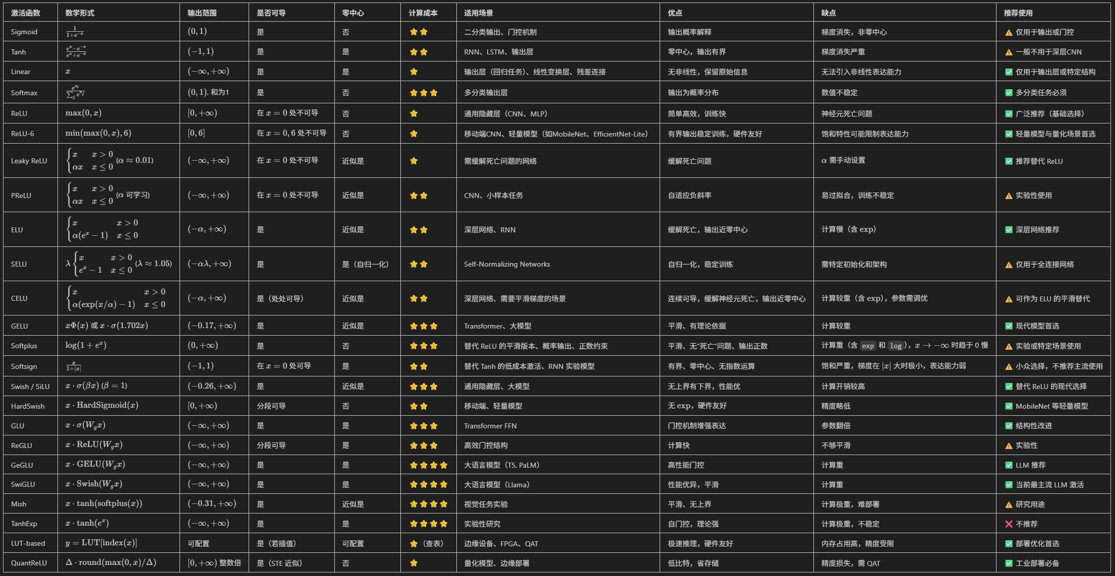
整體對比
下表從數學形式、輸出範圍、是否可導、是否零中心、計算成本、適用場景、優點、缺點等維度,總結了常用的 20 多種激活函數的性質。