

此分類用於記錄吳恩達深度學習課程的學習筆記。
課程相關信息鏈接如下:
- 原課程視頻鏈接:[雙語字幕]吳恩達深度學習deeplearning.ai
- github課程資料,含課件與筆記:吳恩達深度學習教學資料
- 課程配套練習(中英)與答案:吳恩達深度學習課後習題與答案
本篇為第四課第四周的課後習題和代碼實踐部分。
1. 理論習題
【中英】【吳恩達課後測驗】Course 4 -卷積神經網絡 - 第四周測驗
還是比較簡單,我們就不展開了。
2.代碼實踐
【中英】【吳恩達課後編程作業】Course 4 -卷積神經網絡 - 第四周作業
再次提醒 Keras 的導庫問題。
老樣子,我們還是使用現有的成熟框架來分別實現本週介紹的人臉識別和圖像風格轉換模型。
2.1 人臉識別
實際上,在如今的實驗和實際部署中,人臉識別的整套邏輯已經遠比我們在理論部分所介紹的要複雜和完善的多,我們依舊分點來進行介紹。
(1)python 庫:InsightFace
作為一個應用中生活中方方面面的技術,就像我們之前介紹的目標檢測有ultralytics,人臉識別也有將成熟算法體系工程化、模塊化的工具庫:InsightFace
InsightFace 是基於 ArcFace 等先進算法構建的人臉分析庫,功能涵蓋:
- 人臉檢測:支持單人或多人圖像檢測,返回人臉框和關鍵點;
- 人臉對齊:通過關鍵點實現旋轉、縮放等對齊操作,提高識別精度;
- 人臉識別/驗證:提取 embedding,進行相似度計算或一對多搜索;
- 性別、年齡、姿態估計:內置輕量化預測模型;
- 模塊化、可擴展:你可以直接使用預訓練模型,也可以替換為自己訓練的模型。
使用 InsightFace,我們幾乎不需要從零實現算法邏輯,只需調用接口即可完成人臉識別的實驗和演示。
同樣,我們可以通過 pip 安裝 InsightFace 相關依賴:
pip install insightface onnxruntime
其中:
- CPU 版本:默認安裝即可,無需額外配置。
- GPU 版本:如果希望使用 GPU 加速,則需要安裝 GPU 版本 ONNX Runtime:
pip install onnxruntime-gpu
有一些注意事項,如果不進行相關配置會導致報錯:
- ONNX Runtime GPU 需要 CUDA 和 cuDNN 與當前版本兼容
- 在 Windows 上,部分組件需要 Microsoft C++ Build Tools,用於編譯部分 C++/Cython 擴展:
- 安裝 Visual Studio Installer
- 勾選 “使用 C++ 的桌面開發”
- 即可保證
insightface或其他依賴(如face3d)可以正確編譯。
在成功安裝 InsightFace 後,我們來看看如何使用這個框架。
(2)InsightFace 預訓練模型
我們對預訓練模型的使用也早就不陌生了,InsightFace 同樣內置了一系列從輕量級到重量級的預訓練模型,我們可以通過接口實現下載並調用。
來簡單看一段代碼:
from insightface.app import FaceAnalysis
app = FaceAnalysis(name='buffalo_l')  # 會自動下載預訓練模型,這是一種輕量級模型
當你運行時,模型會緩存到用户目錄下,自動下載並解壓,無需手動配置:
C:\Users\<用户名>\.insightface\models\
需要特別説明的是,buffalo_l 模型不僅僅是單一的識別模型,它實際上集成了人臉識別任務中的多個環節,包括:
- 人臉檢測 :在輸入圖像中快速找到人臉區域。
- 關鍵點定位:在檢測到的人臉上標出關鍵點(如眼睛、嘴角、鼻尖等)。
- 3D 人臉建模(可選,部分模型):預測人臉的三維結構信息。
- 人臉特徵提取:將每張人臉映射到一個高維向量空間,就是我們之前説的編碼。
- 性別與年齡預測(部分模型):預測人臉的性別和年齡區間。
瞭解了它的功能後,現在我們就來演示一下:
(3)示例使用:人臉檢測
我們用這樣一段代碼來進行初始化和人臉檢測:
from insightface.app import FaceAnalysis
import cv2 # 用來讀取圖像

app = FaceAnalysis(name='buffalo_l')  # 輕量級預訓練模型
app.prepare(ctx_id=0, det_size=(640, 640))  # ctx_id=-1 使用 CPU
img = cv2.imread("images4.jpg") # 讀取圖片
faces = app.get(img) # 傳入模型進行處理

if faces:
    print("檢測到人臉數量:", len(faces))
    print("第一張人臉 embedding:", faces[0].embedding[:20]) # 只顯示前 20 維
    print("第二張人臉 embedding:", faces[1].embedding[:20])
來看看運行後的效果:
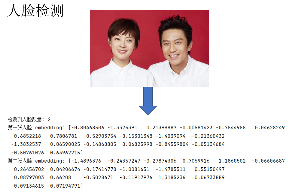
這樣,就完成了對圖像的編碼。
(4)示例使用:關鍵點定位
同樣,只要所選用的預訓練模型支持,app.get(img)的同樣可以實現關鍵點定位:
from insightface.app import FaceAnalysis
import cv2

app = FaceAnalysis(name='buffalo_l')
app.prepare(ctx_id=0, det_size=(640, 640))
img = cv2.imread("images4.jpg")
faces = app.get(img)

if faces:
    # 畫定位圖
    vis = img.copy()
    for face in faces:
        bbox = face.bbox.astype(int)
        cv2.rectangle(vis, (bbox[0], bbox[1]), (bbox[2], bbox[3]), (0, 255, 0), 2)
        if 'landmark_2d_106' in face:
            landmarks_2d = face['landmark_2d_106'].astype(int)
            for (x, y) in landmarks_2d:
                cv2.circle(vis, (x, y), 2, (0, 0, 255), -1)
    # 保存結果
    cv2.imwrite("output.jpg", vis)
    print("結果已保存到 output.jpg")
來看結果:
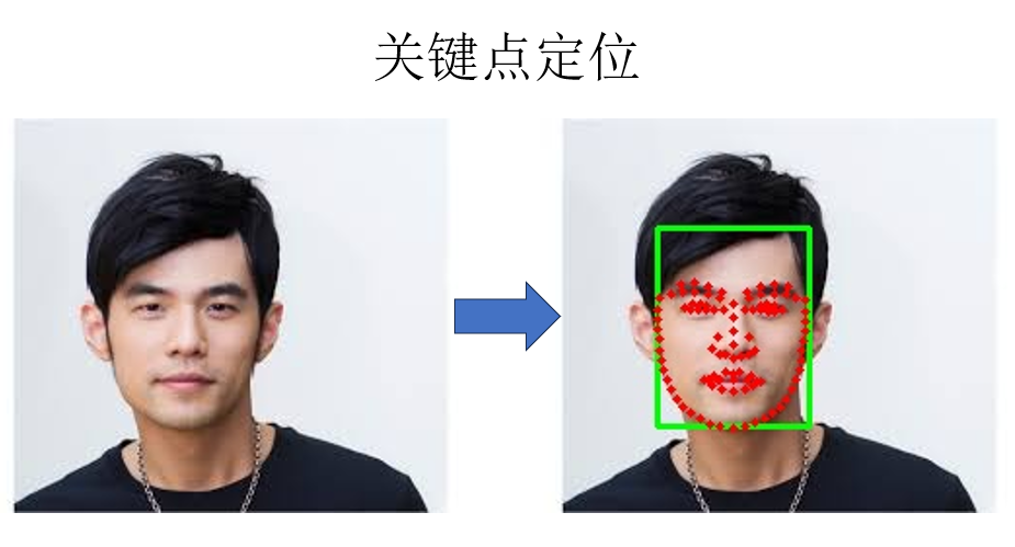
同樣可以較為成功的定位到人臉的各個部位。
(5)通過相似度學習實現人臉識別
演示了一些基本功能後,我們回到正題,再回顧一下原理:人臉識別並非要訓練“你是誰”的網絡,而是“你更像誰”的網絡。即學習相似度而非分類,以此來實現具有較高部署價值的系統。
因此,我們可以把兩幅圖像輸入預訓練模型,通過二者的編碼來計算它們的相似度,代碼如下:
import cv2
import numpy as np
from insightface.app import FaceAnalysis

# 1. 初始化
InsightFaceapp = FaceAnalysis(name='buffalo_l')
app.prepare(ctx_id=-1, det_size=(640, 640))  # ctx_id=-1 用 CPU
# 2. 讀取圖片
img1 = cv2.imread("images1.jpg")
img2 = cv2.imread("images2.jpg")

# 3. 檢測並提取人臉 embedding
faces1 = app.get(img1)
faces2 = app.get(img2)
emb1 = faces1[0].embedding
emb2 = faces2[0].embedding

# 4. 另一種更常用的相似度計算:餘弦相似度
def cosine_similarity(a, b):
    return np.dot(a, b) / (np.linalg.norm(a) * np.linalg.norm(b))
sim = cosine_similarity(emb1, emb2)
print(f"Cosine similarity: {sim:.4f}")

# 5.閾值決策
if sim > 0.60:
    print("很可能是同一個人")
else:
    print("很可能不是同一個人")
來看結果:
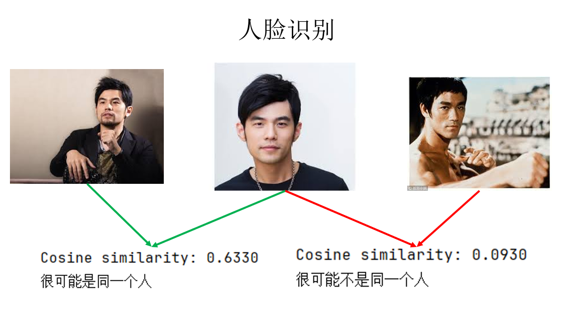
這樣,我們就通過學習相似度,避免了因人數增加而導致的結構和訓練問題,實現了人臉識別。
而在實際應用中,我們便可以將所有識別目標預先輸入模型得到編碼並存儲,與刷臉時截取的圖像輸入模型得到的編碼依次計算相似度,根據結果進行下一步操作。
同時,如果希望得到指標更高的結果,我們可以下載更重量級的模型。
現在還有一個問題:如果我們想自己訓練模型呢?
由於 InsightFace 本身主要是 提供預訓練模型和推理/應用接口,所以它並沒有像 Pytorch 或 TF 一樣完全封裝一套“開箱即用、端到端訓練你自己數據集”的完整訓練流水線。
因此,我們雖然可以調用 InsightFace 定義的網絡結構,但仍需要藉助 Pytorch 或 TF 來編碼數據輸入、訓練和梯度下降等邏輯。
但為了實現二者的兼容使用,我們就又要進行很多設置,一個更常見的思路是完全使用Pytorch 或 TF 來搭建自己的人臉識別網絡,但這又涉及一些我們還沒介紹過的網絡結構。
因此在這裏就不再展開了,在相關理論補充完成後,我們再來進行這部分內容。
下面來看另一部分:圖像風格轉換。
2.2 圖像風格轉換
同樣先回顧一下圖像風格轉換的核心思想:在固定預訓練卷積神經網絡參數的前提下,利用網絡中間層特徵,將圖像的內容結構與風格統計進行顯式分離,並通過在特徵空間中最小化相應的代價函數,直接對輸入圖像進行優化,從而重構出一幅同時匹配內容與風格約束的圖像。
因此,要實現一個圖像風格轉換網絡,我們首先要選擇一個經過預訓練,可以合理提取圖像特徵的網絡作為工具。
在這裏,我選擇使用 VGG16 作為預訓練模型:
vgg = models.vgg16(pretrained=True).features.to(device).eval() # 選擇評估模式
for param in vgg.parameters():  # 凍結所有網絡參數
    param.requires_grad = False
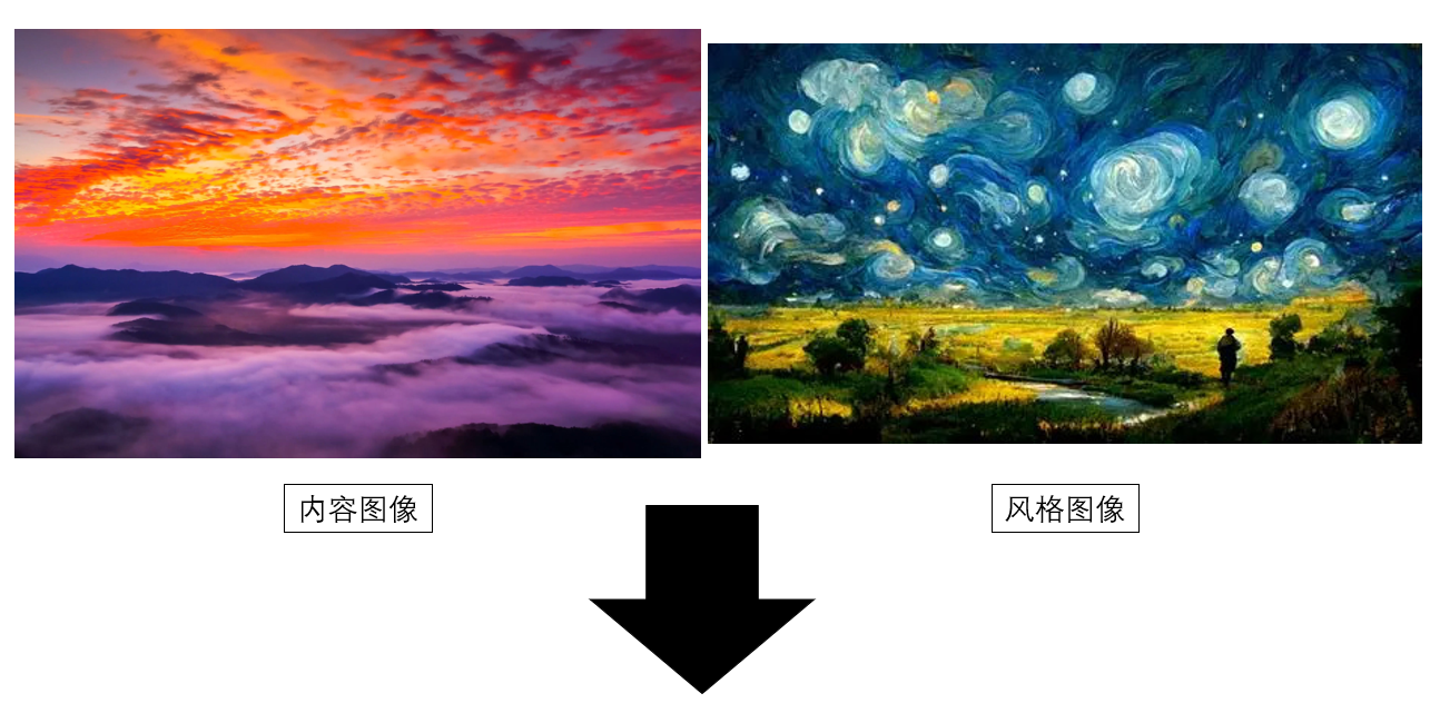
開始編碼,首先,我們需要對風格圖和內容圖兩幅圖像進行處理:
# 讀取並預處理輸入圖像:統一尺寸、轉換為張量並送入指定設備,網絡輸入要求
def load_image(path, size=(512, 256)):
    image = Image.open(path).convert("RGB")
    transform = transforms.Compose([
        transforms.Resize(size),
        transforms.ToTensor()
    ])
    return transform(image).unsqueeze(0).to(device)

content = load_image("content.jpg")
style = load_image("style.jpg")
此外,我們還需要一些工具方法:
# 將模型輸出的張量形式圖像後處理為 PIL 圖像,用於結果可視化與保存
def tensor_to_pil(tensor):
    image = tensor.cpu().clone().squeeze(0)
    image = transforms.ToPILImage()(image.clamp(0,1))
    return image

# 提取輸出特徵圖用於計算代價
def get_features(x, model, layers):
    features = {}
    for name, layer in model._modules.items():
        x = layer(x)
        if name in layers:
            features[name] = x
    return features

# 計算 Gram 矩陣用於計算風格代價
def gram_matrix(features):
    b, ch, h, w = features.size()
    features = features.view(b, ch, h*w)
    gram = torch.bmm(features, features.transpose(1,2))
    return gram / (ch*h*w)
最後,再進行傳播前的超參數設置:
# 指定用於內容表示的 VGG 網絡層(通常選用較深層,保留語義信息)
content_layers = ['15']
# 指定用於風格表示的 VGG 網絡層(從淺到深,捕捉不同尺度的紋理與統計特徵)
style_layers   = ['0', '5', '10', '15']
# 以內容圖像為初始值創建可優化的輸出圖像張量,並開啓梯度計算
output = content.clone().requires_grad_(True).to(device)
# 使用 L-BFGS 優化器對輸出圖像進行優化(風格遷移中常用)
optimizer = optim.LBFGS([output])
# 風格損失的權重,控制生成結果中風格特徵的強度
style_weight = 1e6
# 內容損失的權重,控制生成結果與原內容圖像的相似程度
content_weight = 1
# 提前計算內容圖像在指定內容層上的特徵表示
content_features = get_features(content, vgg, content_layers)
# 提前計算風格圖像在指定風格層上的特徵表示
style_features = get_features(style, vgg, style_layers)
# 提前對風格圖像的各層特徵計算 Gram 矩陣,用於表示風格的統計特性
style_grams = {layer: gram_matrix(style_features[layer]) for layer in style_layers}
# 設置優化的總迭代次數
num_steps = 400
# 設置每隔多少步保存或顯示一次中間結果
display_step = 50
# 用於存儲每隔 display_step 生成的輸出圖像,便於可視化訓練過程
output_images = []
由此,我們終於可以進行訓練了:
run = [0]
while run[0] <= num_steps:
    def closure():
        optimizer.zero_grad()
        output_features = get_features(output, vgg, content_layers + style_layers)

        # 內容損失
        content_loss = 0
        for layer in content_layers:
            content_loss += torch.mean((output_features[layer] - content_features[layer])**2)

        # 風格損失
        style_loss = 0
        for layer in style_layers:
            G = gram_matrix(output_features[layer])
            style_loss += torch.mean((G - style_grams[layer])**2)

        total_loss = content_weight * content_loss + style_weight * style_loss
        total_loss.backward()

        # 保存中間輸出
        if run[0] % display_step == 0:
            print(f"Step {run[0]}: Total Loss: {total_loss.item():.2f}")
            output_images.append(tensor_to_pil(output.clone()))
        run[0] += 1
        return total_loss

    optimizer.step(closure)
現在,來看看結果吧:
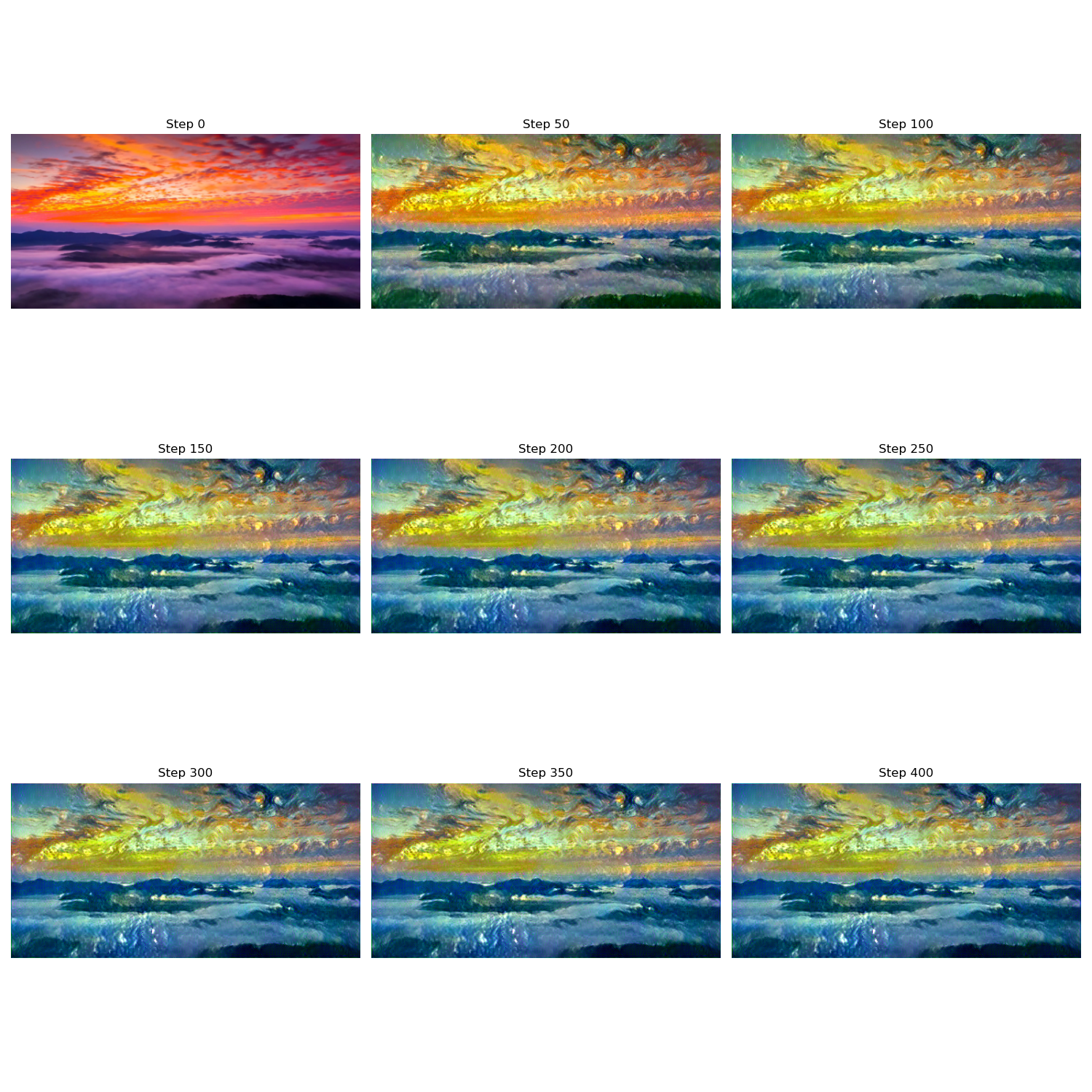
這樣,我們就完成了圖像的風格轉換,你也可以更換為自己的圖像來試試效果。
3. 附錄
3.1 圖像風格轉換代碼 Pytorch版
import torch
import torch.optim as optim
from torchvision import transforms, models
from PIL import Image
import matplotlib.pyplot as plt
device = torch.device("cuda" if torch.cuda.is_available() else "cpu")
print("Using device:", device)
# 讀取並預處理輸入圖像:統一尺寸、轉換為張量並送入指定設備,網絡輸入要求
def load_image(path, size=(256, 512)):
    image = Image.open(path).convert("RGB")
    transform = transforms.Compose([
        transforms.Resize(size),
        transforms.ToTensor()
    ])
    return transform(image).unsqueeze(0).to(device)

content = load_image("content.jpg")
style = load_image("style.jpg")
# 將模型輸出的張量形式圖像後處理為 PIL 圖像,用於結果可視化與保存
def tensor_to_pil(tensor):
    image = tensor.cpu().clone().squeeze(0)
    image = transforms.ToPILImage()(image.clamp(0,1))
    return image
# 計算 Gram 矩陣用於計算風格代價
def gram_matrix(features):
    b, ch, h, w = features.size()
    features = features.view(b, ch, h*w)
    gram = torch.bmm(features, features.transpose(1,2))
    return gram / (ch*h*w)

vgg = models.vgg16(pretrained=True).features.to(device).eval()
for param in vgg.parameters():
    param.requires_grad = False

content_layers = ['15']
style_layers   = ['0','5','10','15']

def get_features(x, model, layers):
    features = {}
    for name, layer in model._modules.items():
        x = layer(x)
        if name in layers:
            features[name] = x
    return features

output = content.clone().requires_grad_(True).to(device)
optimizer = optim.LBFGS([output])

style_weight = 1e6
content_weight = 1

content_features = get_features(content, vgg, content_layers)
style_features = get_features(style, vgg, style_layers)
style_grams = {layer: gram_matrix(style_features[layer]) for layer in style_layers}

num_steps = 400
display_step = 50

# 用於存儲每隔 display_step 的輸出
output_images = []

print("開始優化...")
run = [0]
while run[0] <= num_steps:
    def closure():
        optimizer.zero_grad()
        output_features = get_features(output, vgg, content_layers + style_layers)

        # 內容損失
        content_loss = 0
        for layer in content_layers:
            content_loss += torch.mean((output_features[layer] - content_features[layer])**2)

        # 風格損失
        style_loss = 0
        for layer in style_layers:
            G = gram_matrix(output_features[layer])
            style_loss += torch.mean((G - style_grams[layer])**2)

        total_loss = content_weight * content_loss + style_weight * style_loss
        total_loss.backward()

        # 保存中間輸出
        if run[0] % display_step == 0:
            print(f"Step {run[0]}: Total Loss: {total_loss.item():.2f}")
            output_images.append(tensor_to_pil(output.clone()))
        run[0] += 1
        return total_loss

    optimizer.step(closure)


num_imgs = len(output_images)
cols = 3
rows = (num_imgs + cols - 1) // cols
plt.figure(figsize=(5*cols, 5*rows))
for i, img in enumerate(output_images):
    plt.subplot(rows, cols, i+1)
    plt.imshow(img)
    plt.axis('off')
    plt.title(f"Step {i*display_step}")
plt.tight_layout()
plt.show()
3.2 圖像風格轉換代碼 TF版
import tensorflow as tf
import numpy as np
import matplotlib.pyplot as plt

from tensorflow.keras.applications.vgg16 import VGG16, preprocess_input
from tensorflow.keras.models import Model
from tensorflow.keras.preprocessing import image

def load_and_process_img(path, target_size=None, max_size=512):
    img = image.load_img(path)
    if max(img.size) > max_size:
        scale = max_size / max(img.size)
        img = img.resize((int(img.size[0] * scale), int(img.size[1] * scale)))
    if target_size is not None:
        img = img.resize(target_size)
    img = image.img_to_array(img)
    img = np.expand_dims(img, axis=0)
    img = preprocess_input(img)
    return tf.convert_to_tensor(img, dtype=tf.float32)

device = "/GPU:0" if tf.config.list_physical_devices('GPU') else "/CPU:0"
print("Using device:", device)
content_path = "content.jpg"
style_path = "style.jpg"
max_size = 512
content_weight = 1.0
style_weight = 1e6
num_steps = 400
display_step = 50

content_pil = image.load_img(content_path)
if max(content_pil.size) > max_size:
    scale = max_size / max(content_pil.size)
    final_size = (int(content_pil.size[0] * scale), int(content_pil.size[1] * scale))
else:
    final_size = content_pil.size

print(f"最終統一圖像尺寸: {final_size}")


content_img = load_and_process_img(content_path, max_size=max_size)
style_img = load_and_process_img(style_path, target_size=final_size, max_size=max_size)
vgg = VGG16(include_top=False, weights='imagenet')
vgg.trainable = False

content_layers = ['block4_conv2']
style_layers = ['block1_conv1', 'block2_conv1', 'block3_conv1', 'block4_conv1']

outputs = [vgg.get_layer(name).output for name in (style_layers + content_layers)]
model = Model(vgg.input, outputs)


def gram_matrix(tensor):
    x = tf.transpose(tensor, [0, 3, 1, 2])
    b, c, h, w = tf.shape(x)
    features = tf.reshape(x, (b, c, h * w))
    gram = tf.matmul(features, features, transpose_b=True)
    return gram / tf.cast(c * h * w, tf.float32)

def get_features(x):
    outs = model(x)
    style_outs = outs[:len(style_layers)]
    content_outs = outs[len(style_layers):]
    return style_outs, content_outs


style_features, content_features = get_features(style_img)
style_grams = [gram_matrix(f) for f in style_features]
noise = tf.random.uniform(tf.shape(content_img), -20., 20.)
output_img = tf.Variable(content_img + noise)

optimizer = tf.optimizers.Adam(learning_rate=5.0)
def deprocess_img(x):
    x = x.numpy()[0]
    x[:, :, 0] += 103.939
    x[:, :, 1] += 116.779
    x[:, :, 2] += 123.68
    x = x[:, :, ::-1]  # BGR -> RGB
    x = np.clip(x, 0, 255).astype('uint8')
    return x
output_images = []

for step in range(num_steps):
    with tf.GradientTape() as tape:
        style_out, content_out = get_features(output_img)
        # 內容損失
        content_loss = tf.add_n([tf.reduce_mean((a - b) ** 2)
                                 for a, b in zip(content_out, content_features)])
        # 風格損失
        style_loss = tf.add_n([tf.reduce_mean((gram_matrix(a) - g) ** 2)
                               for a, g in zip(style_out, style_grams)])

        total_loss = content_weight * content_loss + style_weight * style_loss

    grads = tape.gradient(total_loss, output_img)
    optimizer.apply_gradients([(grads, output_img)])

    if step % display_step == 0:
        print(f"Step {step}, Total loss: {total_loss:.2f}")
        output_images.append(deprocess_img(output_img))

num_imgs = len(output_images)
cols = 3
rows = (num_imgs + cols - 1) // cols

plt.figure(figsize=(5 * cols, 5 * rows))
for i, img in enumerate(output_images):
    plt.subplot(rows, cols, i + 1)
    plt.imshow(img)
    plt.title(f"Step {i * display_step}")
    plt.axis('off')
plt.tight_layout()
plt.show()