


前言
孤立森林,一種非常高效快速的異常檢測算法
開始探索
scikit-learn
import numpy as np
import matplotlib.pyplot as plt
from sklearn.ensemble import IsolationForest

rng = np.random.RandomState(0)

X_train = 0.3 * rng.randn(100, 2)
X_outliers = rng.uniform(low=-2, high=2, size=(10, 2))

clf = IsolationForest(n_estimators=100, max_samples='auto', contamination='auto', random_state=rng)
clf.fit(X_train)

y_pred_train = clf.predict(X_train)
y_pred_outliers = clf.predict(X_outliers)

plt.title("Isolation Forest")
plt.scatter(X_train[:, 0], X_train[:, 1], color='b', label="Normal")
plt.scatter(X_outliers[:, 0], X_outliers[:, 1], color='r', label="Outliers")

plt.legend()
plt.axis('tight')
plt.show()
腳本!啓動:

深入理解
類似於隨機森林,但每棵樹不使用信息增益或基尼係數等指標,而是隨機選擇一個特徵,在該特徵的最小值和最大值之間隨機選一個切分值,將數據集分成兩部分,又在每個部分隨機最大值與最小值之間隨機選一個切分支,不斷遞歸。指導到達指定深度或者當前節點只有1個樣本
構造如此的樹n棵,組成森林,開始計算每個樣本在每棵樹的平均路徑長度(葉子節點的深度depth),計算異常分數
- \(s \approx 1\),強異常點,很容易被孤立
- \(0.5 \le s < 1\),可能是異常點,越接近1越是異常點,需要配合其他參數來確定,比如異常點比例
- \(s < 0.5\),正常點
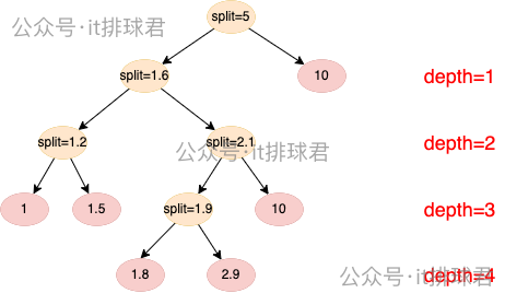
舉例説明
假設有以下樣本: [1, 1.5, 1.8, 2.0, 2.3, 10]
構造第一棵樹:
1)第一層:depth=1,隨機選擇劃分值:1 < split < 10 的區間中選擇 split = 5
- 左子樹:[1, 1.5, 1.8, 2.0, 2.3]
- 右子樹:[10.0]
2)第二層:depth=2,隨機選擇劃分值:1 < split < 2.3 的區間中選擇 split = 1.6
- 左子樹:[1, 1.5]
- 右子樹:[1.8, 2.0, 2.3]
3)第三層:depth=3,左子樹,隨機選擇劃分值:1 < split < 1.5 的區間中選擇 split = 1.2
- 左子樹:[1]
- 右子樹:[1.5]
4)第三層:depth=3,右子樹,隨機選擇劃分值:1.8 < split < 2.3 的區間中選擇 split = 2.1
- 左子樹:[1.8, 2.0]
- 右子樹:[2.3]
5)第四層:depth=4,隨機選擇劃分值:1.8 < split < 2.9 的區間中選擇 split = 1.9
- 左子樹:[1.8]
- 右子樹:[2.9]
6)計算路徑
| 樣本值 | 路徑長度 |
|---|---|
| 1.0 | 3 |
| 1.5 | 3 |
| 1.8 | 4 |
| 2.0 | 4 |
| 2.3 | 3 |
| 10.0 | 1 |
重複構造第n棵樹,得出路徑,計算路徑平均值
| 樣本值 | 第1棵樹路徑 | 第2棵樹路徑 | 第n棵樹路徑 | 平均路徑 |
|---|---|---|---|---|
| 1.0 | 3 | 3 | .. | 3 |
| 1.5 | 3 | 3 | .. | 3 |
| 1.8 | 4 | 4 | .. | 4 |
| 2.0 | 4 | 4 | .. | 4 |
| 2.3 | 3 | 3 | .. | 3 |
| 10.0 | 1 | 1 | .. | 1 |
計算異常得分
1)計算樣本(1.0):
- 樣本長度:\(E(x) = 3\)
- 樣本規模 \(n=6\) 的平均路徑期望:
2)計算所有樣本
| 樣本值 | 平均長度 | 異常得分 |
|---|---|---|
| 1.0 | 3 | 0.4882 |
| 1.5 | 3 | 0.4882 |
| 1.8 | 4 | 0.3844 |
| 2.0 | 4 | 0.3844 |
| 2.3 | 3 | 0.4882 |
| 10.0 | 1 | 0.7874 |
判斷異常點:
- 路徑長度越短的越異常,比如10.0的路徑長度為1,在第一次分割的時候就被孤立了
- 異常分數越高就是異常點
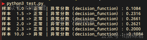
sklearn中的異常分數
from sklearn.ensemble import IsolationForest
import numpy as np

X = np.array([[1], [1.5], [1.8], [2], [2.3], [10]])

clf = IsolationForest(random_state=0, contamination='auto')
clf.fit(X)

pred = clf.predict(X)
score = clf.decision_function(X)

for x, p, s in zip(X, pred, score):
    print(f"樣本 {x[0]:>4} -> {'異常' if p==-1 else '正常'} | 異常分數(decision_function): {s:.4f}")
腳本!啓動:

問題出現了:
- sklearn的分數和手工計算的並不一樣
- 為什麼
1.0被當成異常了 - 分數越小反而越異常
先看第一個問題,sklearn的分數和手工計算的並不一樣。首先,每棵樹是採用部分的樣本來計算,而不是採用所有的樣本n=6來計算的。其次,在上面的手工計算中,期望路徑長度\(c(n)\)中的\(H(n)\),並不是由這個公式計算的
這個公式一旦n的數量增大,\(H(n)\)的計算將會帶來很大的計算消耗,通常使用另外一個公式計算近似值:
以上兩點原因,帶來的就是sklearn計算異常分數與手工計算不一樣
再看第二個問題,為什麼1.0被當成異常了
只需要調整一個參數,contamination=0.1就可以解決這個問題了
contamination用來調節異常比例的參數,如果是auto,那麼異常比例為33.3%,6個樣本,那麼異常點就是2個。手動調整為0.1,那就告訴模型只有1個異常點,那麼最不正常的就是10.0了
最後第三個問題,分數越小反而越異常。這明顯是計算方式不一樣造成的,這裏直接解析一下源碼,版本:scikit-learn:1.6.1:
-
decision_function函數def decision_function(self, X): return self.score_samples(X) - self.offset_ -
score_samples函數返回的是:經過公式\(s(x,n) = 2^{-\frac{E(x)}{c(n)}}\)計算的相反數def score_samples(self, X): ... return self._score_samples(X) def _score_samples(self, X): return -self._compute_chunked_score_samples(X) def _compute_chunked_score_samples(self, X): ... for sl in slices: # compute score on the slices of test samples: scores[sl] = self._compute_score_samples(X[sl], subsample_features) return scores def _compute_score_samples(self, X, subsample_features): ... scores = 2 ** ( # For a single training sample, denominator and depth are 0. # Therefore, we set the score manually to 1. -np.divide( depths, denominator, out=np.ones_like(depths), where=denominator != 0 ) ) return scores -
self.offset_是根據整個樣本異常分數,再加上異常比例參數contamination的中位數計算出來的self.offset_ = np.percentile(self._score_samples(X), 100.0 * self.contamination)
看到這裏,我就想説,複雜就行了,經過這麼複雜的計算,與手動計算出來的肯定不一樣
小結
在sklearn中
- 找到孤立點,
contamination是一個非常重要的參數,它決定了每個節點的分數以及後續確定是否異常 - 快速找到孤立點,直接通過
pred函數即可,-1是孤立點,1是正常點 - 想要獲取點的評分,通過
decision_function函數獲取評分,與理論公式不同,評分越低反而越異常
小結
- 聯繫我,做深入的交流
![]()

至此,本文結束
在下才疏學淺,有撒湯漏水的,請各位不吝賜教...
