


前言
在之前的討論中,討論的都是線性迴歸,自變量與結果可以通過一條直線來解釋。而今天討論的問題,自變量與結果可能需要曲線來擬合,也就是所謂的 \(x^n\),n>=2
開始探索
老規矩,先運行起來,再探索原理
1. scikit-learn
import numpy as np
from sklearn.preprocessing import PolynomialFeatures
from sklearn.linear_model import LinearRegression
from sklearn.pipeline import Pipeline
from sklearn.metrics import mean_squared_error, r2_score
def adjusted_r2(r2, n, p):
return 1 - (1 - r2) * (n - 1) / (n - p - 1)
np.random.seed(0)
x = np.linspace(-5, 5, 50)
y_true = 0.8 * x**2 - 2 * x + 1
y_noise = np.random.normal(0, 1, len(x))
y = y_true + y_noise
model_poly = Pipeline([
('poly', PolynomialFeatures(degree=2)),
('linear', LinearRegression())
])
model_poly.fit(x.reshape(-1, 1), y)
y_pred = model_poly.predict(x.reshape(-1, 1))
r2 = r2_score(y, y_pred)
n = len(x)
p = 2 # 多項式階數
r2_adj = adjusted_r2(r2, n, p)
MSE = mean_squared_error(y, y_pred)
coef = model_poly.named_steps['linear'].coef_
intercept = model_poly.named_steps['linear'].intercept_
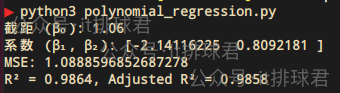
print(f"截距 (β₀): {intercept:.2f}")
print(f"係數 (β₁, β₂): {coef[1:]}")
print("MSE:", MSE)
print(f"R² = {r2:.4f}, Adjusted R² = {r2_adj:.4f}")
腳本!啓動:
2. 報告解讀
又是熟悉的兄弟夥
- MSE:均方誤差,用於衡量模型預測值與真實值之間的差異,越趨於0越好
- R²:決定係數,用於評估模型擬合優度的重要指標,其取值範圍為[0, 1]
- 調整R²:調整決定係數,對R²的修正,懲罰不必要的特徵(防止過擬合)。需要注意的是,這裏計算調整決定係數的時候,p為多項式的階數
在本次測試中,我們已經假定了多項式是: $$0.8x^2 - 2x + 1$$ 而最終模型為$$0.809x^2 - 2.141x + 1.06$$
深入理解多項式迴歸
1. 數學模型
- \(β_0\) 叫做截距,在模型中起到了“基準值”的作用,就是當自變量為0的時候,因變量的基準值
- \(β_1\) \(β_2\) \(\dots\) \(β_n\) 叫做自變量係數或者回歸係數,描述了自變量對結果的影響方向和大小
- 多項式迴歸中,依然使用最小二乘法,是
scikit-learn包的默認算法
- 多項式迴歸中,依然使用最小二乘法,是
2. 損失函數
線性迴歸通常使用均方誤差(MSE)來作為損失函數,衡量測試值與真實值之間的差異
其中\(y_i\)是真實值,\(\hat{y}_i\)是預測值
正如前文提到,MSE中真實值與預測值,有平方計算,那就會放大誤差,所以MSE可以非常有效的檢測誤差項
3. 決定係數
用於評估線性迴歸模型擬合優度的重要指標,其取值範圍為 [0, 1]
其中\(y_i\)是真實值,\(\hat{y}_i\)是預測值,\(\bar{y}\)是均值
scikit-learn中的常用參數
這裏有一個非常重要的參數,degree,這裏表達了用幾階多項式來擬合模型。在本例中,使用的是2階多項式,如果解釋效果不好,可以嘗試高階多項式
如何選擇迴歸模型
觀察數據特徵
最直觀的方法,先將數據做散列點圖,簡單評估一下
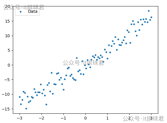
一眼望去,可以用線性迴歸模型
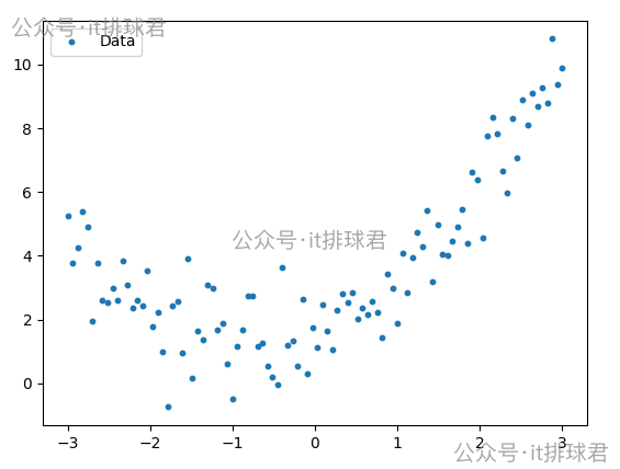
這看起來是一條曲線,可以嘗試用多項式模型
模型評估
先看線性模型與多項式模型的MSE與R²的對比
import numpy as np
from sklearn.preprocessing import PolynomialFeatures
from sklearn.linear_model import LinearRegression
from sklearn.pipeline import Pipeline
from sklearn.metrics import mean_squared_error, r2_score

# 生成數據:y = 0.5x² + x + 噪聲
np.random.seed(0)
x = np.linspace(-3, 3, 100)
y_true = 0.5 * x**2 + x
y = y_true + np.random.normal(0, 1, len(x))  # 添加噪聲

# 線性模型
model = LinearRegression()
model.fit(x.reshape(-1, 1), y)
y_pred = model.predict(x.reshape(-1, 1))
MSE = mean_squared_error(y, y_pred)
r2 = r2_score(y, y_pred)
print("線性模型:")
print("R²:", r2)
print("MSE:", MSE)
print(f"截距 (β₀): {model.intercept_}")
print(f"係數 (β): {model.coef_}\n")

# 多項式模型
model2 = Pipeline([
    ('poly', PolynomialFeatures(degree=2)),
    ('linear', LinearRegression())
])
model2.fit(x.reshape(-1, 1), y)
y_pred = model2.predict(x.reshape(-1, 1))
MSE = mean_squared_error(y, y_pred)
r2 = r2_score(y, y_pred)
print("多項式模型,階數為2:")
print("R²:", r2)
print("MSE:", MSE)
print(f"截距 (β₀): {model2.named_steps['linear'].intercept_}")
print(f"係數 (β): {model2.named_steps['linear'].coef_[1:]}\n")
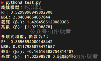
明顯是多項式模型解釋性更好
殘差圖
所謂殘差,是單個樣本點的預測值與真實值之間的差
- \(e_i\):殘差
- \(y_i\):樣本真實值
- \(\hat{y}_i\):樣本預測值
import numpy as np
import matplotlib.pyplot as plt
from sklearn.preprocessing import PolynomialFeatures
from sklearn.linear_model import LinearRegression
from sklearn.pipeline import Pipeline
from sklearn.metrics import mean_squared_error, r2_score

# 生成數據:y = 0.5x² + x + 噪聲
np.random.seed(0)
x = np.linspace(-3, 3, 100)
y_true = 0.5 * x**2 + x
y = y_true + np.random.normal(0, 1, len(x))  # 添加噪聲

def fit_poly(degree):
    model = Pipeline([
        ('poly', PolynomialFeatures(degree=degree)),
        ('linear', LinearRegression())
    ])
    model.fit(x.reshape(-1, 1), y)
    y_pred = model.predict(x.reshape(-1, 1))
    residuals = y - y_pred  # 計算殘差
    return residuals

degrees = [1, 2]

plt.figure(figsize=(15, 4))
for i, degree in enumerate(degrees):
    residuals = fit_poly(degree)
    plt.subplot(1, 2, i+1)
    plt.scatter(x, residuals, s=10)
    plt.axhline(y=0, color='r', linestyle='--')
    plt.title(f"Residual Plots (degree={degree})")
    plt.xlabel("x")
    plt.ylabel("Residual")
plt.show()
注意這裏線性迴歸也可以直接通過指定degree=1來完成
腳本!啓動
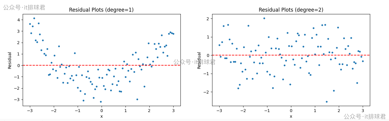
- 左邊是線性迴歸,右邊是2次多項式迴歸
- 線性迴歸的殘差呈現出明顯的
U型,説明未捕獲非線性趨勢 - 2次多項式的殘差隨機分散在0附近,無規律,説明擬合良好
- 正確的殘差圖不僅要體現出隨機性,還要體現不可預測性
階數選擇
import numpy as np
from sklearn.preprocessing import PolynomialFeatures
from sklearn.linear_model import LinearRegression
from sklearn.pipeline import Pipeline
from sklearn.metrics import mean_squared_error, r2_score

# 生成數據:y = 0.5x² + x + 噪聲
np.random.seed(0)
x = np.linspace(-3, 3, 100)
y_true = 0.5 * x**2 + x
y = y_true + np.random.normal(0, 1, len(x))  # 添加噪聲

def adjusted_r2(r2, n, p):
    return 1 - (1 - r2) * (n - 1) / (n - p - 1)

def fit_poly(degree):
    model = Pipeline([
        ('poly', PolynomialFeatures(degree=degree)),
        ('linear', LinearRegression())
    ])
    model.fit(x.reshape(-1, 1), y)
    y_pred = model.predict(x.reshape(-1, 1))
    MSE = mean_squared_error(y, y_pred)
    r2 = r2_score(y, y_pred)
    adj_r2 = adjusted_r2(r2, len(x), degree)
    print(f'階數:{degree},MSE:{MSE},r2:{r2}, adj_r2:{adj_r2}')
    print('=='*10)

degrees = [2, 3, 4, 5]
for i, degree in enumerate(degrees):
    fit_poly(degree)
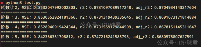
- 通過2-5階的遍歷,發現2階的調整決定係數是最高的
- 通過不斷的升階,雖然決定係數在慢慢上升,但是調整決定係數並沒有上升,所以升階並不能造成模型有實質的改變。這個問題在線性迴歸詳細描述過
- 2階多項式就是擬合度更高的模型
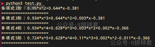
對比:
原始的函數為 \(y=0.5x^{2}+x\) ,通過截距與迴歸係數,計算出不同階的方程,然後與原函數對比
import numpy as np
from sklearn.preprocessing import PolynomialFeatures
from sklearn.linear_model import LinearRegression
from sklearn.pipeline import Pipeline

# 生成數據:y = 0.5x² + x + 噪聲
np.random.seed(0)
x = np.linspace(-3, 3, 100)
y_true = 0.5 * x**2 + x
y = y_true + np.random.normal(0, 1, len(x))  # 添加噪聲

def adjusted_r2(r2, n, p):
    return 1 - (1 - r2) * (n - 1) / (n - p - 1)

def format(args):
    n = len(args)
    terms = []
    for i, coeff in enumerate(args):
        power = n - 1 - i
        if coeff == 0:
            continue
        term = ""
        if coeff > 0 and terms:
            term += "+"
        elif coeff < 0:
            term += "-"
            coeff = abs(coeff)
        if coeff != 1 or power == 0:
            term += str(round(coeff, 3))
            if power > 0:
                term += "*"
        if power > 0:
            term += "x"
            if power > 1:
                term += f"^{power}"
        terms.append(term)
    return "".join(terms) if terms else "0"

def fit_poly(degree):
    model = Pipeline([
        ('poly', PolynomialFeatures(degree=degree)),
        ('linear', LinearRegression())
    ])
    model.fit(x.reshape(-1, 1), y)
    coef = model.named_steps['linear'].coef_
    intercept = model.named_steps['linear'].intercept_
    args = coef[1:].tolist()
    args.append(intercept)
    s = format(args)
    print(f'多項式{degree}階:{s}')
    print('=='*10)

degrees = [2, 3, 4, 5]
for i, degree in enumerate(degrees):
    fit_poly(degree)
進行對比,可以通過該網站畫出函數圖
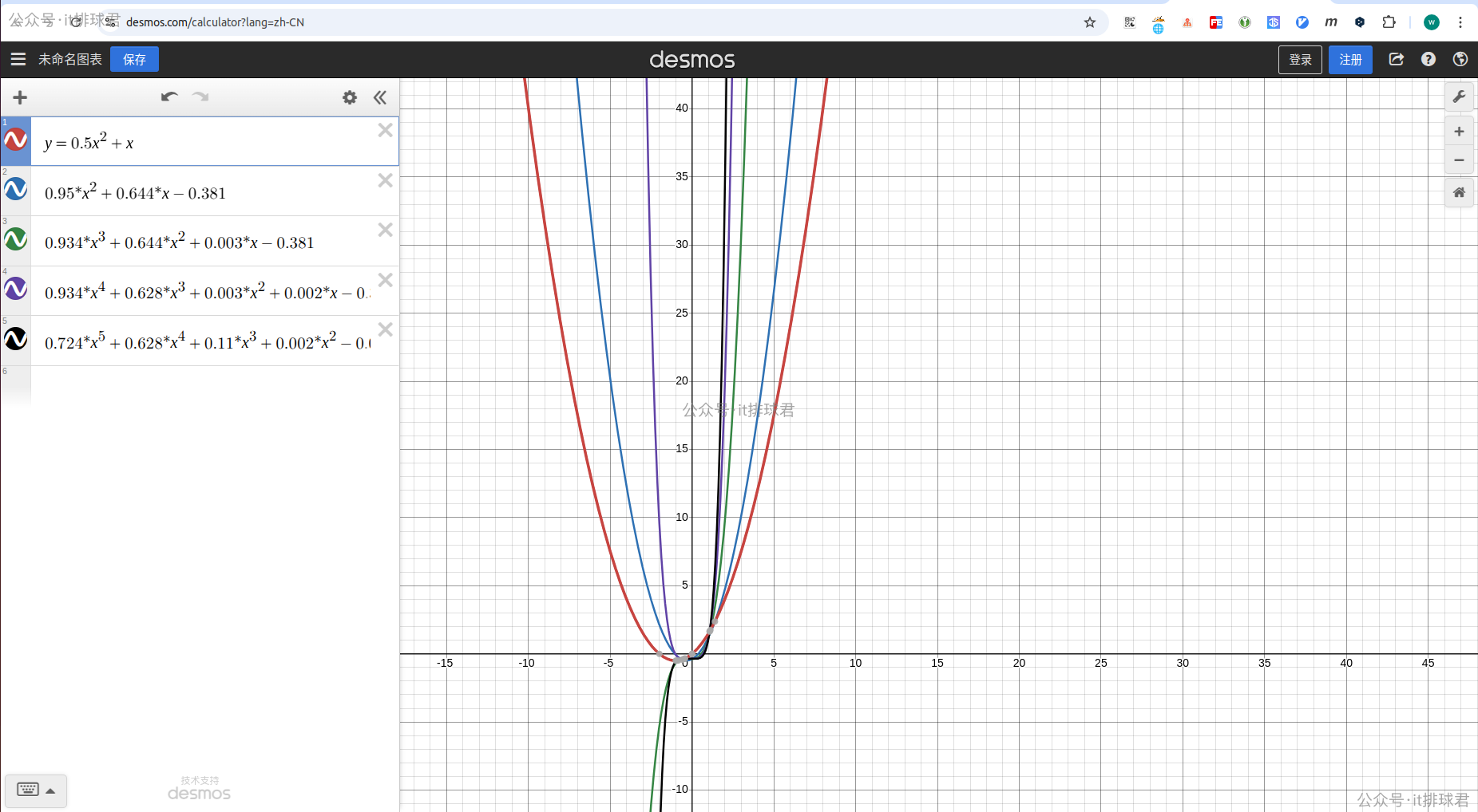
紅色是原二次函數,而藍色是經過噪聲之後擬合的二次函數,與紅色是最接近的,越往Y軸靠,階數越高
pipeline
它可以將多個數據處理步驟和機器學習模型組合成一個整體的工作流
之前在lasso迴歸那裏,在lasso迴歸之前,需要將數據標準化,再進行模型訓練
scaler = StandardScaler()
X_scaled = scaler.fit_transform(X2)

lasso = Lasso(alpha=0.1)
lasso.fit(X_scaled, y2)
通過pipleline,可以直接寫成一個工作流
from sklearn.pipeline import Pipeline

lasso_pipe = Pipeline([
    ('scaler', StandardScaler()),
    ('lasso', Lasso(alpha=0.1))
])

lasso_pipe.fit(X2, y2)
當然還有本次多項式迴歸中提到的
model_poly = Pipeline([
    ('poly', PolynomialFeatures(degree=2)),
    ('linear', LinearRegression())
])
可以看到,先進行PolynomialFeatures,這就是所謂的升階操作,再進行LinearRegression線性迴歸。在sklearn中,多項式的處理方式本質就是先升階,再進行線性迴歸,所以線性迴歸的理論都可以用在多項式迴歸當中
聯繫我
- 聯繫我,做深入的交流

至此,本文結束
在下才疏學淺,有撒湯漏水的,請各位不吝賜教...
